Olivier in Wonderland
The AEA presidential lecture by Olivier Blanchard has become an instant success. In this blog, Charles Wyplosz flags some caveats to bear in mind when interpreting his lecture.
Search the site

The AEA presidential lecture by Olivier Blanchard has become an instant success. In this blog, Charles Wyplosz flags some caveats to bear in mind when interpreting his lecture.
The AEA presidential lecture by Olivier Blanchard (Blanchard 2019) has become an instant success. It suggests that the welfare costs of deficits and debts are smaller than commonly thought. Although it is carefully crafted and merely calls for “a richer discussion”, it is frequently interpreted as a suggestion that deficits and debts do not deserve to be considered as a key concern for policymakers (for instance, on 23 May 2019 the Financial Times ran an article entitled “Top economist says Japan should learn to love budget deficits”). Blanchard is keenly aware of the pitfalls of this conclusion, which takes us back to the naïve macroeconomics of the 1960s when, ignoring the budget constraint, the IS-LM model showed that expansionary fiscal policy is essentially free. The ensuing accumulation of public debts gave Keynesianism a bad name, for good reason. Now, after years of pro-cyclical austerity policies in many of the developed economies, the message is tapping into a well of frustrations and its popular success is disturbing, especially as debt levels are very high in many countries.
This short note is not meant to criticise Blanchard’s contribution per se but to flag and reinforce some caveats, which are mentioned in the lecture. To that effect, I consider a large sample of OECD countries to examine whether the US experience is special.
When the interest rate on the public debt is lower than the GDP growth rate, the debt follows a stable process, with an important implication. The debt-to-GDP ratio tends to decline because borrowing ‘pays for itself’. This is not new, of course. The additional twist is that, historically in the US, the interest rate has often been lower than the growth rate. In addition, current forecasts are that this situation will last, and not just in the US. While it lasts, governments should not be mesmerised by their debt levels and could use the budget to stabilise the economy when it is slowing down and to undertake productive public investments.
The process driving the public debt is on the following accounting identity:
Bt+1 – Bt = (rt – gt) Bt + Dt
where Bt is the public debt at the end of period t, Dt is the period’s primary budget deficit, both as a proportion of GDP, while rt and gt are, respectively, the nominal interest and the growth rate of nominal GDP.
This identity makes it clear that benign neglect of the debt rests on a number of assumptions:
This note argues that these hypotheses are not warranted. To that effect, I have collected data for the OECD countries1 for the period since 1961. This choice is motivated by data availability. Even so, the sample starts later for many countries. Gross debt ratios are provided by the IMF historical debt database, ten-year interest rates come from the OECD and GDP from the World Bank’s World Development Indicators. This provides 895 annual observations for 22 countries.
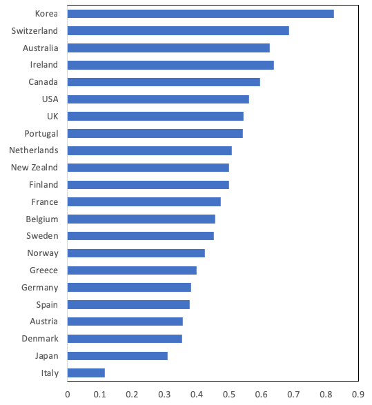
Observations with r -g < 0 represent 49.7% of the sample. Country details are shown in Figure 1. Even in the US, which is not the country with the highest proportion of occurrences, r – g < 0 happened in 56.1% of the years.2 The average differential for the whole sample stands at 0.10%, with a large standard deviation of 4.36 (more about this below).
During and after the global financial crisis, many central banks drove their interest rates down to the perceived effective lower bound, and they are still there almost a decade later. In fact, over the period ending in 2007, the proportion of observations where r – g < 0 is slightly lower at 47.9%. The reason is that nominal growth has also declined even more than the interest rate.
Figure 1 Proportion of years when r – g < 0


Blanchard is more careful than me about the interest rate that he uses. He makes two seemingly desirable adjustments, which I cannot do on my multi-country dataset. First, he notes that the one-year interest rate is usually significantly lower than the ten-year rate used here, which biases r – gupward. His interest rate is the weighted average of one-year and ten-year interest rates with weights computed to match the – changing – average maturity of the debt. The importance of this adjustment is not as obvious as it seems. That r – g < 0 alleviates the budget constraint rests on the view that the existing debt is rolled over as need when it matures. Maturing debt instruments are replaced by newly created instruments, as long as needed. For example, a one-year bond will be replaced n times over n years. Under the interest rate term structure assumption, an n-year interest rate compounds n successive one-year rates, and the n-year rate correctly captures the rollover process. The rate that should be used, then, is the interest rate of bonds that mature at the end of the horizon (which, in theory, is infinite). Of course, this argument faces two pitfalls. First, long interest rates are compounded on the basis of expectations of future short rates, which are likely to prove wrong. Consequently, the term structure assumption may fail to capture the actual evolution of the debt. Second, the term structure assumption, as stated, ignores the term and risk premia, which goes a long way toward explaining why long rates typically exceed short rates. I return to this important issue in Section 4.
Blanchard also correctly notes that the returns on privately held bonds are taxed, which provides income for the government or, equivalently, reduces the interest cost r. Using a unique feature of the US tax code,3 he can compute the effective tax rate, which he deducts from r. This helps make occurrences of r – g < 0 more frequent. However, the tax receipts affect the budget balance and should therefore be deducted from the government income. Blanchard recognises this point but, as noted above (Section 2) and below (Section 4), he does not consider the evolution of the budget deficit. Whether tax receipts appear in the term (r – g)B of in D in the debt accounting identity is immaterial if we consider the budget deficit.
As noted above, the standard deviation of r – g is very large. Statistically, this means that it is impossible to make inferences about whether r – g is negative or positive as a ‘norm’.
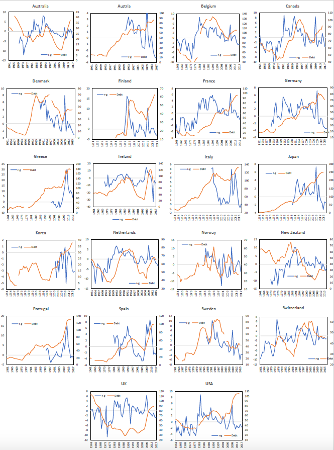
A quick look at Figure 2, which displays the evolution of r – g (left scale) and of the debt ratio (right scale) in the sample countries, reveals that, in the past, across OECD countries the sign of r – g has gone through swings, sometimes at relatively low frequency. When the interest differential shifts from negative to positive, the debt accumulation process switches from stable to unstable. If the debt is large and/or if there is a sizeable primary deficit, the debt then tends to increase fast, as both debt service and the primary balance work in the same direction. Allowing the primary budget to go negative while ignoring the debt level when r – g < 0 is dangerous in a world where governments are unable or unwilling to promptly offset changes in debt service. Concerns for debt stability are as important in good years, when r – g < 0, as they are in bad years, when r – g > 0, unless we are sure that r – g < 0 is indeed the norm.
Ignoring the evolution of the primary balance amounts to implicitly assuming that the budget balances are independent of the (adjusted) debt service. This question immediately reminds us of the deficit bias hypothesis. A voluminous literature, starting with Alesina and Tabellini (1990), Alesina and Drazen (1991) and von Hagen and Harden (1995), shows that governments tend to pay insufficient attention to the longer run implications of budget deficits. A biased government sets the overall deficit Bt+1 – Bt too high, irrespective of its two components. Thus, when r – g becomes negative, the debt-to-GDP ratio tends to decline, which biased governments may see as an opportunity to raise the deficit. When and if r – g subsequently becomes positive, the government may fail to react soon enough and strongly enough to stem the debt increase.
I am not aware of a systemic analysis of the two-way relationship between r – g and D. There is a sizeable literature on whether large deficits or debts raise the interest rate, including the term and risk premia. Some authors have detected a significant effect (e.g. Laubach 2009), but they do not look at the interest differential r – g. Following Bohn (1998), there is also a large literature on the reaction of the deficit to the debt, which generally finds that governments cut deficits when the debt rises, in effect stabilising the debt accumulation process. However, the large increases of public debts over the last decade indicate that this virtuous behaviour cannot be taken for granted, especially when low growth worsens both the debt service and the primary deficit through reduced tax income. With both r – g and D endogenous to a wide variety of shocks, it is going to be very difficult – but most helpful – to determine whether D is reduced, and by how much, when r – gswitches from negative to positive.
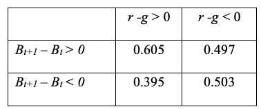
Short of such an analysis, it may be useful to look at the data. Figure 2 shows that, in some cases (Finland, the Netherlands, Spain) the debt declines almost only and always when r – g < 0, but in most other cases there is no visible link. The average of country correlations between rt – gt and the deficit Bt+1 – Bt is 0.332, which confirms that a declining interest differential helps reduce the debt ratio, but it also means that debt increases ominously when the differential rises. On the basis of the sample, Table 1 indicates what happens to the debt when the sign of r – g changes. The debt decreases more often than it increases when r – g < 0, but just about (50.3% of the time). When r – g > 0, it rises more often (60.5%). This shows that the primary budget matters. To make matters worse, as recognised by Blanchard, self-fulfilling crises are a serious threat. If, for some reason, the markets interpret a large debt and/or lasting sizeable deficits as a risk of debt default, the interest rate can quickly rise and either force a costly abrupt deficit retrenchment or a provoke a full-blown crisis, possibly both. This is one lesson from the European debt crisis and from instabilities in many countries, as is well documented (Reinhart and Rogoff 2009). In the presence of a deficit bias, the debt ratio may grow even when r – g < 0 (about half of the time in the sample). Then when the debt is high and markets get worried, r – g becomes positive and governments react with their fastest option. They raise taxes, which precipitates the economy into a recession that is much deeper than had the adjustment come mostly through spending cuts, particularly spending on pensions (see Alesina et al. 2019).
Table 1 Proportion of deficit changes depending on the sign of r – g


It is tempting to follow Blanchard as he suggests that it is a good time to carry out debt-financed productive public investment spending when r – g < 0. In a world where when r – g < 0 is not the norm, and instead fluctuates, what would that imply for the conduct of fiscal deficit? Rigorously examining the cyclical behaviour of r – g is of obvious interest but beyond the scope of this note. Figure 2 displays the correlation coefficients between r – g and the output gap (from the IMF’s World Economic Outlook database) over 1980-2017. With few exceptions, the coefficient is negative; the average over all countries is -0.360. If indeed r – g is countercyclical, governments that follow the suggestion would increase their deficits when the output gap is positive and, conversely, reduce their deficits when the output gap is negative, which means procyclical fiscal policies.
Figure 2 Correlation coefficients r – g and output gap


There is no disagreement that the countercyclical use of fiscal policy stands to improve welfare, but debt build-up works in the opposite direction. It would be wonderful if this trade-off could be eliminated with a systematically negative interest differential. A quick look at the data, however, suggests that r – g < 0 is not the norm and that this alignment of stars fails to systematically reduce the debt ratio. The deficit bias leads to excessive primary deficits and to delayed or misguided government reactions when the sign of r – g switches from negative and positive. In addition, raising the deficit when r – g is low and actual GDP is above potential, and vice versa, would imply that fiscal policy is procyclical. Even worse, perhaps, is the fact that r – g is endogenous to the size of the debt.
It is true that r – g has been negative in recent years in most countries, but the past does not suggest that this will last in the future. The secular stagnation hypothesis argues that the past is a poor guide to the future, but it remains just that – a hypothesis. In addition, even if it were true, there is no guarantee that the interest rate would be on average lower than the reduced growth rate. The world of finance could become dangerous if governments were to believe that we live in the wonderland where the budget constraint does not bite. Blanchard is well aware of these caveats and should not be held responsible for misguided interpretations of his lecture. This note is merely a contribution to the discussion that he calls for.
Figure 3 Public debt and r – g in the 22 sample countries

Author’s note: I am grateful to Olivier Blanchard and Francesco Giavazzi for helpful comments and suggestions.
Alesina, A and A Drazen (1991) ,“Why Are Stabilizations Delayed”, American Economic Review 81: 1170-88.
Alesina, A and G Tabellini (1990), “A Positive Theory of Fiscal Deficits and Government Debt”, The Review of Economic Studies 57(3): 403–414.
Alesina, A, C Favero and F Giavazzi (2019), Austerity, Princeton University Press.
Barrett, P (2018) “Interest-Growth Differentials and Debt Limits in Advanced Economies”, IMF Working Paper WP/18/82.
Blanchard, O (2019), “Public Debt and Low Interest Rates”, American Economic Review,forthcoming.
Bohn, H (1998), “The Behavior of U.S. Public Debt and Deficits”, The Quarterly Journal of Economics 113(3): 949-963.
Laubach, T (2009), “New Evidence on the Interest Rate Effects of Budget Deficits and Debt”, Journal of the European Economic Association 7(4): 858–885.
Mehrotra, N R (2018), “Implications of Low Productivity Growth for Debt Sustainability”, unpublished paper, Brown University.
Mauro, P and J Zilinsky (2016), “Government Debt Ratios in an Era of Low Growth”, Policy Brief 16-10, Peterson Institute for International Economics.
Summers, L H (2015), “Demand Side Secular Stagnation”, American Economic Review 105(5): 60-65.
von Hagen, J and I J Harden (1995), “Budget Processes and Commitment to Fiscal Discipline”, European Economic Review 39 (3-4): 771-779.
[1] A number of countries are excluded: the former Soviet bloc countries and the more recent OECD members. The sample includes: Australia, Austria, Belgium, Canada, Denmark, Finland, France, Germany, Greece, Ireland, Italy, Korea, Netherlands, New Zealand, Norway, Portugal, Spain, Sweden, Switzerland, the UK and the US.
[2] Blanchard quotes three papers that look at international interest differentials and their implication for public debts, Mauro and Zilinsky (2016), Barrett (2018) and Mehrotra (2018). I do not read these papers as backing the claim that r -g < 0 is the norm and that benign neglect of the debt is warranted.
[3] AAA municipal bonds are exempt from Federal taxes, so the difference between their interest rates and those on federal bonds, which are taxed, provides a measure of the effective tax rate.
252 Reads