Identifying overvalued residential house prices has become an integral part of macro-financial surveillance. In light of the lessons learnt from the Global Crisis, detecting boom-bust dynamics in the housing sector in a timely manner is key to preserving macro-financial stability (e.g. Case and Shiller 1989, 2003). To this purpose, metrics aimed at assessing whether house prices are fairly valued are routinely computed and used by surveillance and policy institutions (e.g. ESRB 2015).
House price statistics being available mostly in the form of price indexes excludes direct cross-country comparisons (as opposed to, for example, the Big Mac index comparing the cost of living in different countries). Moreover, existing methods to assess the potential overvaluation of house prices are typically based on differences to historical averages (of ratios such as price to income or price to rental, or fixed effects in regressions-based house price benchmarks based on fundamentals).1 However, the assumption that long-term averages of price indexes represent a reliable reference point may not hold if available time series are short, non-stationary, or characterised by atypical developments, and the cross-country comparison of such misalignment measures becomes problematic whenever time series are of different length.
To fill this gap, in this column we detail the construction of a database covering a number of advanced and emerging economies and providing information on the price per square metre of housing, using a common baseline methodology, and our main insights. Details regarding the construction of the dataset and the properties of house price level estimates are found in Bricongne et al. (2019).2
A database of house price level estimates
The baseline methodology builds price-level data using actual transactions rather than prices asked for by owners and reported by realtors, thereby limiting the risk of overvaluation bias. The price level data are obtained as the ratio of an estimate of the total value of dwellings and associated land to the total floor area of dwellings. Hence, this is a direct top down estimation of the average price per square metre of housing. The sources used for the total value of dwellings are generally national accounts; those for total floor area are census data.3
The baseline estimation approach has a number of advantages. The price level estimate is based on a large sample, thus overcoming possible sample biases of estimates based on surveys, and reflects market transactions rather than prices asked by sellers. The aggregation of prices into a single indicator is obtained on the basis of the number of existing dwellings, thus overcoming the limitation of estimates based on sale offers, which reflect housing market turnover (normally higher in large urban areas). The baseline method has been used for most EU countries and more than 80% of the countries in the sample.
To ensure sufficient country coverage and estimates for all EU countries, in the cases where the baseline estimation method cannot be implemented due to missing data, estimates are obtained using a bottom-up fall-back methodology based on sales offers on the websites of real estate agents, and by turning price averages at sub-regional level into country-level averages.4
By estimating price levels using both the baseline and the fall-back methodology for a number of countries, it is possible to check how large the discrepancies are. The median level of upward bias arising from the use of property advertisements rather than transactions can then be computed and used as a correction factor to improve the comparability of data obtained by the two methods. The corresponding bias is non-negligible but quite limited, the median difference being equal to 7% and the highest one to 12%.
Price level estimates have been computed for 40 countries, referring to years within the 2009-2016 period, depending on the country. Whole time series have subsequently been constructed using house price indexes.
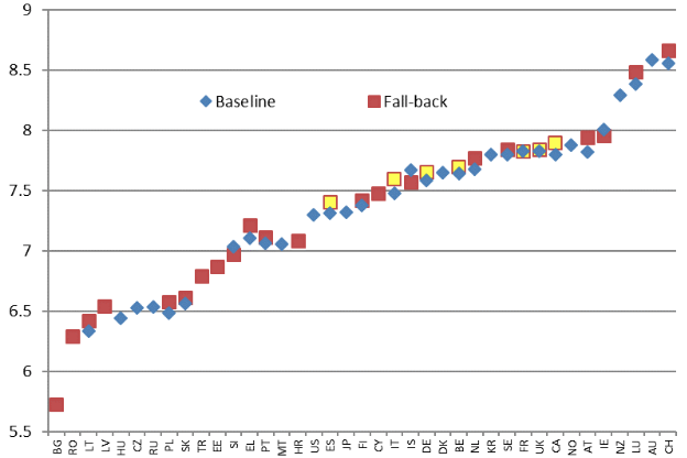
The comparison of the baseline vs. the fall-back method is displayed in Figure 1 for year 2016, pointing to relatively limited cross-country comparability issues despite the different methods.
Figure 1 Prices level estimates in euro per m2, baseline and unadjusted fall-back method, log scale, 2016
Source: Bricongne et al. (2019).
Note: Hong Kong data are not reported because they are out of scale.
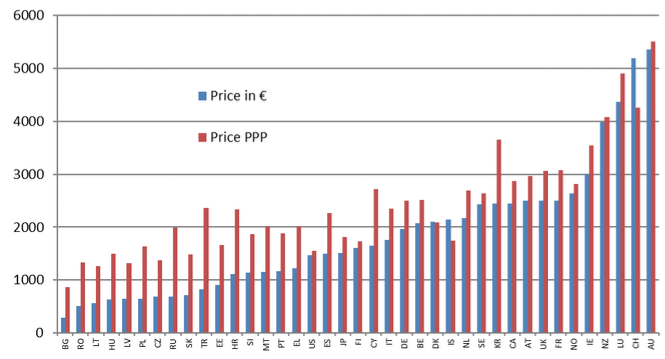
Figure 2 reports price per square metre both in euros and in PPPs. Differences across countries appear broadly to reflect differences in per-capita income. Differences range from around €300/m2 in Bulgaria up to more than €5,000/m2 in Australia in 2016. A number of Eastern European countries display house price levels at the bottom of the cross-country ranking, while particularly high prices are recorded in Hong Kong Luxembourg, Switzerland, and New Zealand.5 Rankings are not much altered when using PPP-converted data.
Figure 2 Price level estimates, prices per m2 in 2016, in € and in PPP (purchasing power parity, PPP = 1 for the US)
Source: Bricongne et al. (2019).
Note: Estimates obtained with the fall-back methodology are corrected to adjust for downward bias. Countries are ranked by increasing order with respect to prices expressed in euros. Hong Kong data are not reported because they are out of scale.
Insights from estimates of house price in levels
Relating house prices to households' income allows for a first assessment of housing affordability. Price level data allow a direct cross-country comparison of price-to-income (PTI) ratios, which would not be possible on the basis of house price indexes.
We compute PTI data as the number of years of income needed to buy an average dwelling of 100 square metres.
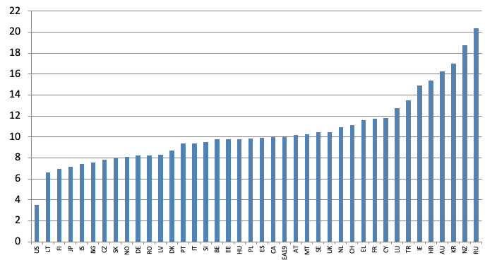
Results are displayed in Figure 3, which provides several insights. First, PTI ratios vary quite a lot, ranging from below 4 years for the US up to around 20 years for Russia. Second, despite such variations, for a majority of countries the PTI ratio is not far from the median value (about 10). Third, PTI ratios display a rather weak relation to income per capita, despite housing being generally considered a superior good, with prices reacting more than proportionally to income. Thus, other relevant factors contribute to differences in PTI. Finally, cross-country rankings in PTI ratios from level data are generally correlated with those from valuation gaps obtained as PTI deviations from country-specific averages from index data, but with notable exceptions.6
Figure 3 Price-to-income ratios (number of yearly incomes required to purchase a 100 m2 dwelling), 2016
Sources: Bricongne et al. (2019).
Note: Estimates obtained with the fall-back methodology are corrected to adjust for downward bias. Countries are ranked by increasing order with respect to prices expressed in euros. Hong Kong data are not reported because they are out of scale.
We also construct early-warning thresholds to detect housing market crashes based on the signalling approach (Kaminsky et al. 1998) and compare the performance of such thresholds using PTI ratios from level data with those computed using valuation gaps from price index data.
Interestingly enough, the PTI threshold that maximises signal power in predicting large downward price corrections is close to the cross-country median value of the PTI.7 In other words, if purchasing a 100 square metre large house requires more than 10 years of income, there is concrete risk of a significant downward correction of house prices in the following three years.
Thresholds obtained from PTI data from levels point to a signal power at least as high as that obtained from metrics built from price indexes irrespective of sample size, while indicators based on indexes need sufficiently long periods to get a high signal power.8
Overall, cross-country consistent price level estimates appear to improve the basis for macro-surveillance of housing issues and to construct a wide range of useful indicators, notably in the implementation of fiscal and macro-prudential policies aimed at addressing potentially harmful house price dynamics.
Authors’ note: The views expressed in the text are the private views of the authors and may not, under any circumstances, be interpreted as stating an official position of the European Commission or Banque de France. We thank Fatoumata Diakhaby for checking the article, through the platform www.b2ideas.eu.
References
Bricongne, J-C, A Turrini, and P Pontuch (2019), “Assessing House Prices: Insights from HouseLev, a Dataset of Price Level Estimates”, European Commission, European Economy Discussion Paper no. 101.
Case, K, and R Shiller (2003), “Is There a Bubble in the Housing Market?”, Brookings Papers on Economic Activity, 2:2003, 299-362.
Case, K, and R Shiller (1989), “The Efficiency of the Market for Single-Family Homes”, American Economic Review, 79 (1), 125-137.
Dujardin, M, A Kelber, and A Lalliard (2015), “Overvaluation in the housing market and returns on residential real estate in the euro area: insights from data in euro per square metre”, Banque de France, Quarterly Selection of Articles, 37, 49-63.
ESRB (2015), “Report on residential real estate and financial stability in the EU”, December.
Girouard, N, M Kennedy, P van den Noord, and C André (2006), “Recent house price developments: the role of fundamentals”, OECD Economics Department Working Papers no. 475.
Kaminsky, G L, S Lizondo, and C M Reinhart (1998), “Leading indicators of currency crises”, IMF Staff Papers vol. 45, no. 1.
Philiponnet, N, and A Turrini (2017), “Assessing House Price Developments in the EU”, European Economy, Discussion Paper no. 48, May.
Endnotes
[1] See, e.g., Girouard et al. (2006) for a survey of alternative approaches to assess house price misalignment.
[2] Available on the link: https://ec.europa.eu/info/publications/assessing-house-prices-insights-h.... See Bricongne et al. (2019) for a detailed description of the data.
[3] In some cases, what is available are individual transaction data rather than information on the aggregate value of dwellings. In such cases, estimates of average price levels have been constructed
[4] Data from realtors' website have been collected via web scraping algorithms with respect to both price and floor area. To ensure that collected data are sufficiently representative, following the rule of thumb in existing estimations of house price levels from transaction data (e.g., Dujardin et al., 2015) the number of observations collected for each country corresponds to a coverage around 1% of the total stock of dwellings present in the country. The degree of geographical disaggregation at which price levels are computed differs across countries and depends on the level of disaggregation of floor area census data.
[5] Hong Kong data are not reported in the graph being an outlier with prices above 30000 €/m2),
[6] For instance, high valuations gaps on the basis of index data found for Sweden and the UK (e.g., Philiponnet and Turrini, 2017) are not matched by particularly high PTI ratios from level data.. Comparatively high PTI ratios from levels for countries like Ireland or Croatia appear at odds with recent moderate or negative valuation gaps based on index data.
[7] The threshold that maximises the signal power is the one that minimises the sum of the shares of missed crises and false alerts. The crisis indicator is defined as a cumulated fall of at least 5% (with a possible exception for one year) in house prices.
[8] Price to income indicators obtained from house price index data are constructed as differences from long-term averages. The signal provided by the indicator depends therefore on the extent to which the long-term average is informative, which depends on sample size.


