‘Leaning against the wind’ (of asset prices and credit booms) is a monetary policy with a somewhat higher policy interest rate than what is justified by just achieving the inflation target and stabilising the real economy without taking any effects on financial stability into account. It has obvious costs in terms of a weaker economy with higher unemployment and lower inflation. It has been justified as a way of reducing the probability and severity of a future financial crisis (Bank for International Settlements 2014 and 2015, Olsen 2015, Sveriges Riksbank 2013). A worse macro outcome in the near future is then considered to be an acceptable cost to be traded off against a better expected macro outcome further into the future. But a crisis can come any time, and the cost of a crisis is higher if initially the economy is weaker. If the unemployment rate is higher when a crisis occurs, the unemployment rate during the crisis will be higher, which increases the cost of a crisis. Leaning against the wind thus not only has costs in terms of a weaker economy if no crisis occurs; it has an additional cost in terms of an even higher cost of a crisis if a crisis occurs. In a new paper (Svensson 2016), I show that, with this additional cost of the policy, for existing empirical estimates its cost exceeds the benefit by a substantial margin.1
‘Leaning against the wind’ policy and its implications
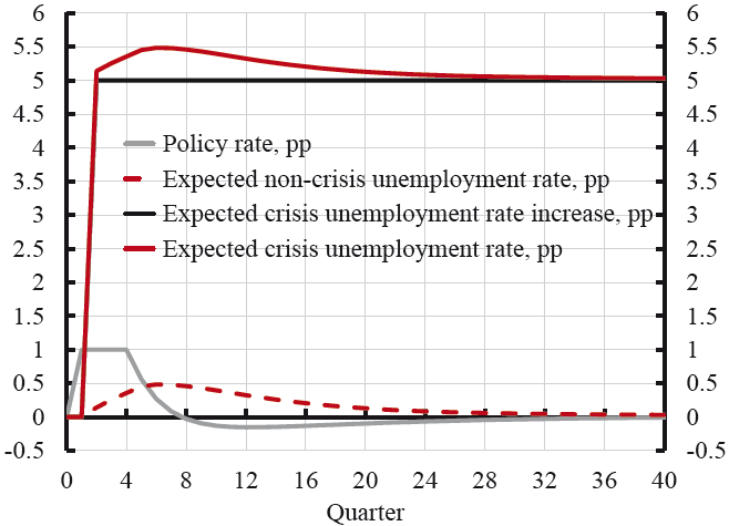
Figure 1. The policy rate, the non-crisis unemployment rate, and the crisis unemployment rate (deviations from baseline)
The dashed red line in Figure 1 shows a typical effect on the future unemployment rate of a policy rate increase of 1 percentage point (pp) during Q1-4, if no crisis occurs.2 The non-crisis unemployment rate increases from the baseline by up to 0.5 percentage points in Q6, and then slowly falls back to the baseline. The solid red line shows the effect on the crisis unemployment rate, that is, the unemployment rate if a crisis occurs and the unemployment rate is assumed to increase by 5 percentage points in a crisis.3 If a crisis would, for instance, occur in Q12, the unemployment rate would increase from the non-crisis unemployment rate of 0.3% to the crisis unemployment rate of 5.3%. The leaning against the wind policy thus increases both the non-crisis and crisis unemployment rate. An increase in the crisis unemployment gap is much more costly than an increase in the non-crisis unemployment gap, also when it is weighted by the probability of a crisis. This has been overlooked by the previous literature mentioned in footnote 1.4
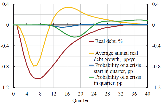
Figure 2. The effect of real debt, annual real debt growth, the probability of a crisis start, and the probability of a crisis of a policy-rate increase of 1 pp during Q1-4
According to Schularick and Taylor (2012), the probability of a crisis starting depends on five lags of annual real debt growth. In Figure 2, the red line shows the effect of the policy rate increase on real debt according to Sveriges Riksbank (2014a). Real debt falls by about 1% relative to the baseline and then rises back to baseline. There is thus monetary neutrality and no permanent effect on real debt. The yellow line shows the effect on the annual growth rate of average annual debt. The growth rate falls below baseline by 0.8 pp in quarter six, but then rises and moves above the baseline after Q11. According to them, the probability of a crisis start depends mostly on real debt growth lagged two years. The blue curve shows the resulting effect on the probability of a crisis start. Because real debt growth has a negative peak in Q6 and a positive peak in Q16, the probability of a crisis starting will have a negative peak in Q14 and a positive peak (barely visible) in Q24.
The green line shows the probability of a crisis in a given quarter. A crisis is assumed to last for eight quarters. Then, the probability of a crisis in a given quarter is equal to the probability of a crisis starting in any of the previous eight quarters. Thus, the green line is a trailing eight-quarter moving sum of the blue line. We see that the probability of a crisis has a negative peak in Q18. However, the effect on the probability of a crisis turns positive after Q24 and stays positive through Q40.5
Because of monetary neutrality, lower real debt growth is followed by higher growth, and the decrease in the probability of a crisis relative to baseline is followed by an increase. There is no effect on the long-run average probability of a crisis; the probability is simply redistributed across periods.
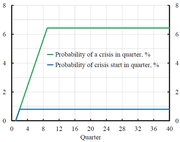
Figure 3. The probability of a crisis starting and the probability of a crisis in a given quarter, under the assumption of a crisis length of eight quarters and conditional on no crisis in Q1
The blue line in Figure 3 shows the assumed benchmark probability of a crisis start in a given quarter, 0.8 pp.6 This means a crisis starts on average every 31 years. The green line shows the probability of a crisis in a given quarter under the assumption of a crisis length of eight quarters, conditional on no crisis in Q1. It equals the sum of the probabilities of crisis starts during the previous eight quarters. The steady-state benchmark probability of a crisis in a given quarter is then 8 x 0.8 = 6.4%.
Calculating marginal costs and benefits from the policy-rate increase
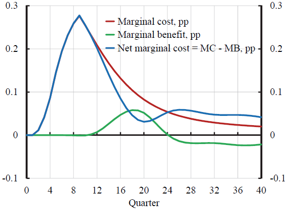
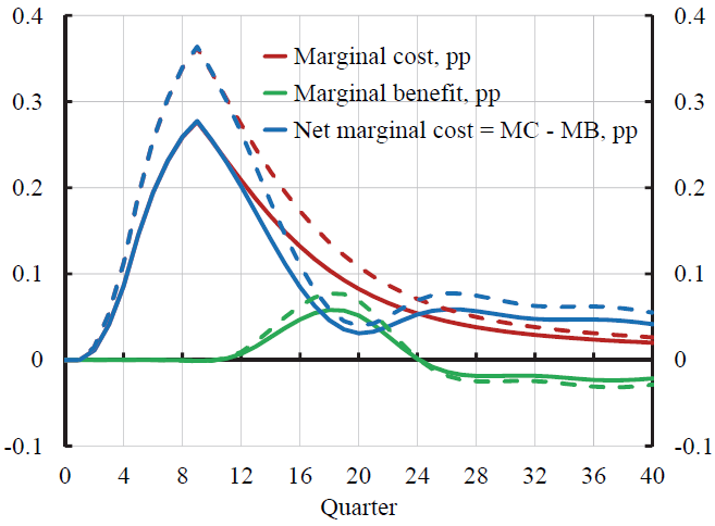
Figure 4. The marginal cost, the marginal benefit, and the net marginal cost of a policy rate increase of 1 pp during Q1-4
Given the information in Figures 1-3, it is possible to calculate the marginal cost and benefit of the policy-rate increase. The red line in Figure 4 shows the marginal cost. It equals the probability-weighted increased crisis loss. The increased crisis loss is due to the crisis starting from a higher non-crisis unemployment rate because of the policy-rate increase, illustrated in Figure 1. The probability is the probability of a crisis in a given quarter, the green line in Figure 3.
The green line in Figure 4 shows the marginal benefit. It consists of the reduction in the expected crisis loss due to the reduction in the probability of a crisis shown in Figure 2. With a quadratic loss function, the crisis loss is the squared crisis unemployment gap, and the marginal benefit is the product of the reduction in the probability of a crisis in Figure 2 and the crisis loss. Because there is an increase rather than a reduction in the probability of a crisis after Q24, the marginal benefit is actually negative after Q24.
The red line shows the net marginal cost, the difference between the red and the green lines. We see that the net marginal cost stays positive for all quarters. The total net marginal cost is the (discounted) sum of the net marginal cost, that is, the (discounted) area under the blue curve. It is clearly positive by a substantial margin.
- It follows that the marginal cost of the leaning against the wind policy dominates the marginal benefit by a large margin.
Because of monetary neutrality, the positive marginal benefit during Q12-24 is followed by a negative marginal benefit thereafter. If, instead, monetary policy is assumed to be non-neutral and has a permanent effect on real debt, the marginal cost would still exceed the marginal benefit by a substantial margin.7
Figure 5. The annual probability of a crisis starting as function of real debt growth during the previous five years
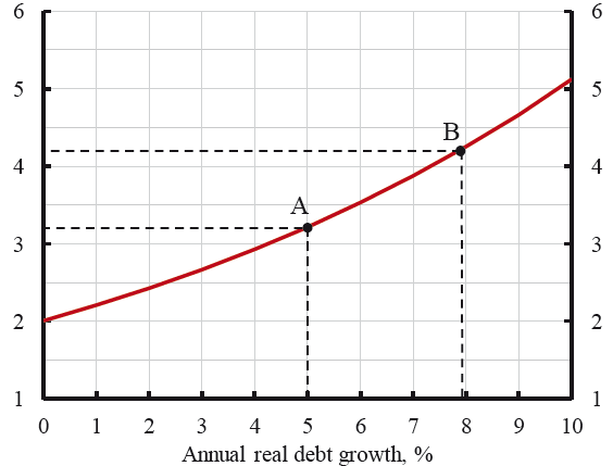
Figure 5 shows the relation between the annual probability of a crisis start and the (steady) real debt growth rate during the previous 5 years according to Schularick and Taylor (2012). The benchmarks 0.8 and 3.2 of, respectively, the quarterly and annual probability of a crisis starting are consistent with 5% real debt growth, corresponding to point A. In order to examine the impact of less effective macroprudential policy on the costs and benefits of leaning against the wind, let me assume that it results in higher real debt growth and a higher annual probability of a crisis starting equal to 4.2%, corresponding to point B. At a higher real debt growth rate, the probability of a crisis starting is also more sensitive to changes in the real debt growth rate.
Figure 6. The effect on the marginal cost, marginal benefit, and net marginal cost of a higher probability of a crisis starting and a higher sensitivity of the probability to real debt growth (dashed lines) compared to the benchmark (solid lines).
The higher probability of a crisis starting implies a higher steady-state probability of a crisis, 8.4%. The higher probability of a crisis implies that the marginal cost, the probability-weighed increased crisis loss, is higher. It is shown as the dashed red line in Figure 6. The higher sensitivity of the probability of a crisis to real debt growth implies that also the marginal benefit is higher (the dashed green line). But we see that the increase in the marginal cost is larger than the increase in the marginal benefit, and the net marginal cost (the dashed red line) increases.
Concluding remarks
Less effective macroprudential policy, or more generally a credit boom, actually makes the case against leaning against the wind policy stronger, not weaker. This obviously runs counter to the common argument that the policy may be justified when macroprudential policy is less effective or even non-existent.
The results reported here are robust to a number of alternative assumptions, as detailed in Svensson (2016). In summary, no support for leaning against the wind is found, even under assumptions strongly biased in favour of it. A minimal policy conclusion is that no leaning against the wind should be undertaken without the support of a thorough cost-benefit analysis. Given the strong case found against leaning against the wind, it seems that the burden of proof should be on its advocates. Another policy conclusion is that, when it comes to reducing the probability or severity of a financial crisis, so far there seems to be no choice but to use policies other than monetary policy, such as micro- and macroprudential policy, housing policy, or fiscal policy, depending on the nature of the problem. Monetary policy is not the right tool.
References
Ajello, A, T Laubach, D Lopez-Salido, and T Nakata (2015), “Financial Stability and Optimal Interest-Rate Policy,” Working paper, Federal Reserve Board, available at www.frbsf.org.
Bank for International Settlements (2014), 84th Annual Report, Bank for International Settlements.
Bank for International Settlements (2015), 85th Annual Report, Bank for International Settlements.
Diaz Kalan, F, S Laséen, D Vestin, and A Zdzienicka (2015), “Leaning Against the Wind: A Note on Costs and Benefits,” Working Paper, International Monetary Fund, forthcoming.
Ekholm, K (2013), “Stabiliseringspolitiken och arbetslösheten (Stabilization Policy and Unemployment, in Swedish),” Presentation at LO, Stockholm, June 19, 2013, Sveriges Riksbank, available at www.lo.se.
IMF (2015), “Monetary Policy and Financial Stability,” Staff Report, International Monetary Fund.
Olsen, Ø (2015), “Integrating Financial Stability and Monetary Policy Analysis,” Speech at the London School of Economics, London, April 27, 2015, Norges Bank.
Schularick, M, and A M Taylor (2012), “Credit Booms Gone Bust: Monetary Policy, Leverage Cycles, and Financial Crises, 1870-2008,” American Economic Review 102, 1029-1061.
Svensson, L EO (2014), “Inflation Targeting and ‘Leaning Against the Wind’,” International Journal of Central Banking 10(2), 103–114.
Svensson, L E O (2015), “Inflation Targeting and Leaning Against the Wind,” in Fourteen Years of Inflation Targeting in South Africa and the Challenge of a Changing Mandate: South African Reserve Bank Conference Proceedings 2014, South African Reserve Bank, 19–36, available at www.larseosvensson.se.
Svensson, L E O (2016), “Cost-Benefit Analysis of Leaning Against the Wind: Are Costs Larger Also with Less Effective Macroprudential Policy?” IMF Working Paper WP/16/3, www.imf.org.
Sveriges Riksbank (2013), “Financial Imbalances in the Monetary Policy Assessment,” box in Monetary Policy Report July 2013.
Sveriges Riksbank (2014a), “The Effects on Monetary Policy on Household Debt,” box in Monetary Policy Report February 2014.
Sveriges Riksbank (2014b), Monetary Policy Report February 2014, Sveriges Riksbank.
Footnotes
1 This additional cost of the leaning against the wind policy has been overlooked by previous work on its cost and benefit , such as Ajello et al. (2015), Diaz Kalan et al. (2015), and IMF (2015), including my own work Svensson (2014, 2015). Even so, this previous work generally finds that the cost of the policy is in most cases several times larger than the benefit. Ajello et al. (2015) find that the optimal amount of leaning against the wind is positive but very small, only a few basis points. With its additional cost, the optimal policy would instead be a modest leaning with the wind.
2 The figure shows the impulse response in the Riksbank’s main model Ramses of the unemployment rate that was reported by Riksbank deputy governor Karolina Ekholm in Ekholm (2013). It is the same response as the one reported to alternative policy-rate paths for quarters 1–12 in Sveriges Riksbank (2014b).
3 This is is the same assumption as the one made in Sveriges Riksbank (2013).
4 With a standard quadratic loss function, in a non-crisis, an unemployment gap of 0.3% instead of zero implies a 0.32 = 0.09 higher non-crisis loss. In a crisis, an unemployment gap of 5.3% instead of 5% implies a 5.32 – 52 = 28.1 – 25 = 3.1 higher crisis loss. That is, the increase in the crisis loss is 3.1/0.09 = 34 times larger than the increase in the non-crisis loss.
5 This is due to the 5-year lagged effects in Schularick and Taylor (2012) estimates.
6 It is consistent with the estimates of Schularick and Taylor (2012) and an average annual real debt growth of 5%, as shown in Figure 5.
7 This would in Figure 2 correspond to real debt (the red line) staying constant at -1% after Q8 and annual real debt growth going back to zero in Q12 and staying at zero thereafter. Then the marginal benefit in Figure 4 would not be negative after Q24 but slightly positive up to Q36, due to the 5-year lag in the Schularick and Taylor (2012) estimates.
