The economics profession did not and does not agree on one question that is critical in the evaluating governments’ responses to the crisis: How large is the stimulus impact of fiscal spending?
In a January 2009 Wall Street Journal op-ed piece, Robert Barro argued that peacetime fiscal multipliers are essentially zero. Christina Romer (2009), Chair of President Obama’s Council of Economic Advisers, used multipliers as high as 1.6 in estimating the job gains that will be generated by the $787 billion stimulus package approved by Congress in February. The difference between Romer’s and Barro’s views of the world amounts to a staggering 3.7 million jobs by the end of 2010.
If anything, the uncertainty regarding the size of fiscal multipliers in developing and emerging markets is even higher. A history of fiscal profligacy and spotty debt repayments calls into question the sustainability of any fiscal expansion. How does this financial fragility affect the size of fiscal multipliers? Does the exchange regime matter? What about the degree of openness? These are all critical policy questions that remain largely unanswered.
New evidence from new data
Data has long been the big hurdle to obtaining precise estimates of fiscal multipliers. In CEPR Policy Insight No. 39, we present our estimates of the fiscal multipliers for developed and emerging economies using new quarterly data for 45 countries (20 high-income and 25 developing) spanning 1960 through 2007. Using this, we estimated fiscal multipliers for different groups of countries.1 The main results are presented in more detail in our Policy Insight. Here is a brief summary of the highlights:
- The response of output to increases in government spending is smaller on impact and considerably less persistent in developing countries than in high-income countries.
- Fiscal multipliers are much larger in economies operating under predetermined exchange rate regimes than under flexible exchange rates.
- Relatively closed economies have much larger multipliers than relatively open economies.
- The output response to increases in government spending is short-lived and much less persistent in highly indebted countries than in countries with a low debt to GDP ratio.
- The multipliers for the US in the post-1980 period are small both in the short and long-run. On the other hand, multipliers for government investment are large.
High-income versus developing countries
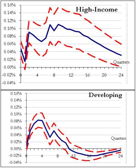
Figure 1 shows the impulse response of GDP to a 1% shock to government consumption; dashed lines indicate the one-standard deviation band. While the impact response is higher in high-income countries (0.05%) than in developing countries (0.01%), the most striking difference is how much more persistent the output response is for high-income countries.
Based on the impulse response depicted in Figure 1, we can compute the corresponding fiscal multipliers. The impact multiplier for high-income countries is 0.24.2 For developing countries, the impact multiplier is close to zero.
Figure 1. Output response to a 1% shock to government consumption
Cumulative multipliers
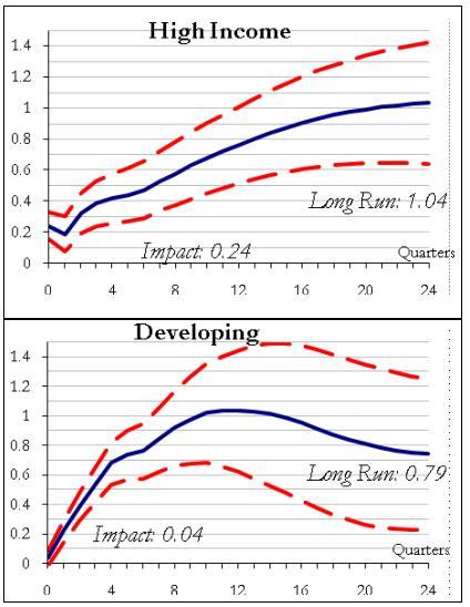
Focusing on the impact multiplier, however, may be misleading because fiscal stimulus packages can only be implemented over time and the economy may only respond gradually. For both groups, Figure 2 shows the cumulative multipliers, defined as the cumulative change in GDP divided by the cumulative change in government consumption (as a percentage of GDP). For example, a value of 0.5 in the third quarter would indicate that, after three quarters, the cumulative increase in output, in dollar terms, is half the size of the cumulative increase in government consumption. The plots also include the value of the long-run cumulative multiplier.3
Figure 2. Cumulative multipliers in response to a shock to government consumption
The cumulative multiplier for high-income countries rises from an initial value of 0.24 (the impact effect) to a long-run value of 1.04; for developing countries it is just 0.79. In other words, in developing countries, an additional dollar of government consumption crowds out some other component of GDP (investment, consumption, or net exports) by 21 cents in the long run.
Exchange rate regimes matter
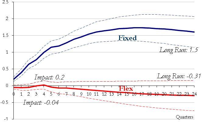
As a second cut at the data, we divided our sample of 45 countries into those with predetermined exchange rates and those with more flexible exchange rate regimes.4 Figure 3 shows the cumulative impulse responses, plainly illustrating the critical role played by the exchange rate regime.
- Under predetermined exchange rates, the impact multiplier is 0.2 (and significantly different from zero) and rises all the way to 1.5 in the long-run.
- Under flexible exchange rate regimes, however, the multiplier is indistinguishable from zero both on impact and in the long run.
Figure 3. Cumulative multipliers: Predetermined and flexible exchange rate regimes
These results are very reminiscent of standard Mundell-Fleming model reasoning – fiscal policy is more effective under predetermined exchange rates because the former regime allows for monetary policy accommodation while the latter does not.
Open versus closed economies
As a third cut at the data, we divided our sample of 45 countries into “open” and “closed” economies.5 The cumulative responses, shown in Figure 4, indicate that the degree of openness is a critical determinant of the size of the fiscal multiplier. For the closed economies, the impact response is 0.26 and reaches 1.6 in the long run. For the open economies, on the other hand, both the impact and the long-run response are not significantly different from zero.
Figure 4. Cumulative multipliers: Open and closed economies
These results are, in principle, consistent with a standard Keynesian view of the world in which the multiplier is lower in a more open economy as a larger fraction of the fiscal expansion is diverted to the rest of the world through higher imports.
Our Policy Insight takes a closer look at various other groupings, including high-versus-low-debt nations, and the US. We present corresponding graphics and analysis for those dimensions.
For the US, we find the impact multiplier is 0.64 and the long-run cumulative multiplier is 1.19. While these estimates are certainly closer to Romer’s than to Barro’s, they mask some important structural changes over the sample period. When estimating the multipliers for the pre-1980 period, we get considerably larger numbers than the post-1980 multipliers. The post-1980 multipliers are just 0.32 on impact and 0.4 in the long-run. This is certainly a far cry from the impact multiplier (1.05) and long-run multiplier (1.55) used in the Romer report.
Conclusions
Our findings lead to the usual “it depends” answer to the size of the fiscal multiplier question. As those familiar with macroeconomic theory likely anticipated, the size of the fiscal multipliers critically depends on key characteristics of the economy (closed versus open, predetermined versus flexible exchange rate regimes, high versus low debt) or on the type of aggregate being considered (government consumption versus government investment). Policymakers would therefore be well-served in taking into account a given country’s characteristics in evaluating the benefits of any fiscal stimulus package.
Footnotes
1 Technically, we have estimated a vector autogression model using the cyclical components of GDP and government consumption. Our identifying assumption, following Blanchard and Perotti (2002), is that discretionary government consumption can only respond to output with a one quarter lag.
2 To arrive at the impact multiplier for, say, high income countries, we simply divide the impact effect in Figure 1 (0.05%) by the ratio of government consumption to GDP (0.21), which gives us 0.24.
3 The long-run multiplier is the value that the cumulative multiplier takes once the responses of both GDP and government consumption have died down. Notice that this may not coincide with the value of the cumulative multiplier after 24 quarters, when our plots end.
4 We followed the updated Reinhart-Rogoff classification in Ilzetzki, Reinhart, and Rogoff (2009).
5 For our purposes, we defined as “open” a country whose foreign trade (imports plus exports) exceeds 60% of GDP and “closed” otherwise. Using this criterion, 29 countries are classified as open and the remaining 16 are classified as closed.
References
Barro, Robert (2009), “Government spending is no free lunch,” Wall Street Journal, 22 January .
Blanchard, Olivier and Roberto Perotti (2002), “An empirical characterization of the dynamic effects of changes in government spending,” Quarterly Journal of Economics pp. 1329-1368.
Ilzetzki, Ethan, Carmen Reinhart and Kenneth Rogoff (2009), “Exchange Rate Arrangements Entering the 21st Century: Which Anchor Will Hold?” mimeo (University of Maryland and Harvard University).
Perotti, Roberto (2004), “Estimating the effects of fiscal policy in OECD countries,” mimeo (Bocconi University).
Romer, Christina, and Jared Bernstein (2009), “The job impact of the American recovery and reinvestment plan,” Council of Economic Advisers, January.


