Perhaps the most important statistic in the design of macroeconomic stabilisation policy is the unemployment gap. This is defined as the distance between the current unemployment rate and the socially efficient unemployment rate. This statistic indicates how far economic activity is from where it should be. Governments strive to reduce the unemployment gap using an array of stabilisation policies, such as monetary policy and fiscal policy.
Once the world emerges from its coronavirus quarantine and economic activity resumes, policymakers will need to assess the unemployment gap. The gap itself will inform governments how much inefficient slack remains within their economies, and how much stabilisation policies need to be brought to bear as a result.
There are currently two measures of the unemployment gap, but neither incorporates an appropriate estimate of the efficient unemployment rate — that is, an indication of where the economy ‘should’ be. The first measure is the difference between actual unemployment and its secular trend. The US Congressional Budget Office produces such a measure. However, this statistic is flawed because trend unemployment is generally not efficient (Pissarides 2000). The second measure used is the difference between actual unemployment and the non-accelerating inflation rate of unemployment (NAIRU), obtained by estimating a Phillips curve linking unemployment and inflation. This measure is flawed as well because the NAIRU does not indicate labour-market efficiency (Rogerson 1997).
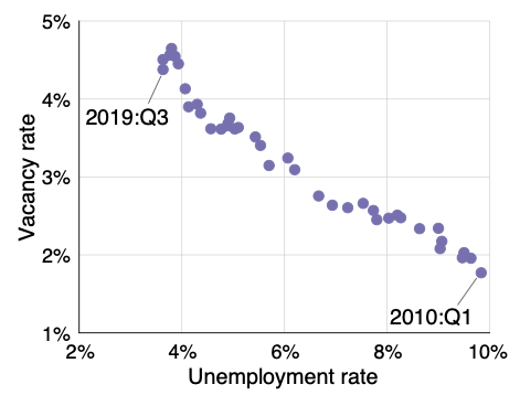
In recent work (Michaillat and Saez 2020), we propose a new and simple measure of the unemployment gap that leverages the modern theory of labour-market efficiency developed by Hosios (1990), built around the Beveridge curve. The Beveridge curve is a mainstay of modern labour markets. It shows that there are few job vacancies when unemployment is high, and that, conversely, there are many job vacancies when unemployment is low. First identified by William Beveridge (in the UK in 1944), it has since been observed in many countries, including the US (Elsby et al. 2015). The US Beveridge curve for the 2010s is presented in Figure 1. There are several theoretical reasons behind the Beveridge curve, but all say roughly the same thing: to maintain a stable employment level when there are fewer unemployed workers looking for jobs, it is necessary to advertise more job vacancies.
Figure 1 Beveridge curve in the United States, 2010–2019
Note: The unemployment rate is constructed by the Bureau of Labor Statistics from the Current Population Survey. The vacancy rate is the number of job openings measured by the Bureau of Labor Statistics in the Job Opening and Labor Turnover Survey, divided by the civilian labor force constructed by the Bureau of Labor Statistics from the Current Population Survey. The unemployment rate is available at https://fred.stlouisfed.org/series/UNRATE; the number of job openings is available at https://fred.stlouisfed.org/series/JTSJOL; and the size of the labor force is available at https://fred.stlouisfed.org/series/CLF16OV.
The Beveridge curve is key to determining the socially efficient unemployment rate because it governs the welfare tradeoff between unemployment and job vacancies. Both unemployment and vacancies come with welfare costs. More unemployment means fewer people are in work and hence fewer productive resources are utilised. In turn, more vacancies mean more productive resources are diverted into recruitment. The Beveridge curve shows that both factors cannot be reduced at the same time: less unemployment requires more vacancies, and fewer vacancies create more unemployment. Our analysis resolves this tradeoff, characterising precisely where the economy should be on the Beveridge curve.
We find that the unemployment gap can be measured from current unemployment and vacancy rates, combined with three statistics: the slope of the Beveridge curve, the average recruiting cost in the economy, and the social value of unemployment relative to employment. These statistics determine the marginal welfare cost and benefit from changing unemployment, and ultimately illustrate the efficient rate of unemployment. For example, consider a small decrease in unemployment. On the positive side, market production mechanically increases. At the same time, newly employed workers forgo home production or leisure, but they also avoid the costs typically associated with being unemployed (such as poorer mental health). Then, on the negative side, more vacancies are required to sustain lower unemployment, as described by the Beveridge curve. This then forces firms to allocate more workers to recruitment processes, reducing overall production. We obtain our formula from the condition that when unemployment is efficient, the positives and negatives balance each other out.
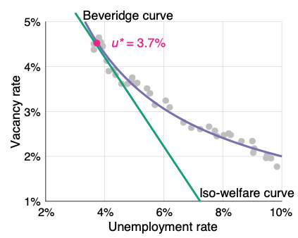
Our method for computing the socially efficient unemployment rate is illustrated in Figure 2, where we apply it to the US during 2010–2019. We find that the efficient unemployment rate is around 3.7%, meaning that the unemployment gap was around zero at the end of 2019 (before the coronavirus crisis started). We arrive at that number by finding the point where the Beveridge curve (purple curve) is tangent to the iso-welfare curve (green line). The iso-welfare curve shows the combinations of unemployment and vacancy rates that provide the same social welfare. Its slope is determined by the recruiting cost and the value of unemployment. This means that higher recruiting costs means that vacancies are costlier from a social perspective, so the curve is flatter. It follows that a higher value of unemployment means that unemployment is less costly from a social perspective, so the curve is also flatter in this case.
Figure 2 Socially efficient unemployment rate in the United States in the 2010s
Note: The Beveridge curve is estimated from the data presented in figure 1. The slope of the iso-welfare curve requires an estimate of the average recruiting cost in the economy, and an estimate of the social value of unemployment relative to employment. We estimate the recruiting cost from the 1997 National Employer Survey, in which the Census Bureau asked 4,500 establishments about their recruiting process and found that firms spend 2.5% of their labor costs on recruiting (Villena Roldan 2010). We estimate the value of unemployment from the work of Borgschulte & Martorell (2018), who use military administrative data for 1993–2004 to determine how servicemembers' choice between reenlisting and exiting the military is affected by the unemployment rate in the local labor market where they would enter. They estimate that the nonpecuniary value of unemployment (through leisure and home production) is 24% of the potential earnings from employment.
The tangency point indicates efficiency for a simple reason. Since both unemployment and vacancies impose a welfare cost, it is preferable for the iso-welfare curve to be as close to the origin of the unemployment-vacancy graph as possible. That being said, the iso-welfare curve has to intersect the Beveridge curve, since the Beveridge curve shows the combinations of unemployment and vacancy rates that are feasible in the economy. Therefore, the furthest inside that the iso-welfare curve can go is at the tangency point with the Beveridge curve.
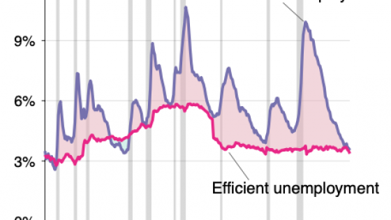
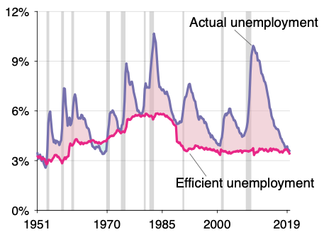
How does the unemployment gap vary over a longer period in the US? Applying the same method, we construct a series for the efficient unemployment rate going back to 1951 (Figure 3). We find that the efficient unemployment rate started at around 3% in the 1950s, steadily climbed to almost 6% in the 1980s, fell just below 4% in the early 1990s, and then remained at that level until 2019. These variations are caused by shifts of the Beveridge curve.
Figure 3 Unemployment gap in the United States, 1951–2019
Note: This graph extends the analysis of figure 2 to the 1951–2019 period. The estimates of the recruiting cost and social value of unemployment are the same as in figure 2. The source of the unemployment rate is the same as in figure 1. The vacancy rate for the 1951–2019 period comes from Barnichon (2010).
Hence, it is clear that the US unemployment gap is almost always positive. The US labour market does not generally operate efficiently but tends to be inefficiently slack. The unemployment gap is especially high in slumps: as high as five percentage points in 1982, 3.9 points in 1992, and 6.2 points in 2010. Thus, historically, it was warranted to implement stabilisation policies that reduced unemployment during difficult times.
In returning the discussion to the upcoming coronavirus recession, macroeconomic theory offers formulas showing that stabilisation policies should move in tandem with the unemployment gap (see Michaillat and Saez (2014) for monetary policy, and Michaillat and Saez (2019) for fiscal policy). Plugging the estimate of the unemployment gap at the onset of the recession into these formulas could help policymakers decide how much they should reduce interest rates (if the zero lower bound is not binding), or how much they should increase public expenditure to combat the crisis.
Finally, in looking to the future we currently have good measures of unemployment and vacancies in the US, but we have much less evidence on the recruiting cost and value of unemployment relative to employment. To improve future measurements of the unemployment gap, it would help to have more evidence on these two statistics. Measuring the evolution of the recruiting cost should be simple. This could be achieved by adding new questions into the Bureau of Labor Statistics’ Job Opening and Labor Turnover Survey or asking firms to report the number of man-hours devoted to recruiting each month, in addition to the number of vacancies. Obtaining more estimates of the value of unemployment might be feasible but is less urgent because the value of unemployment only has a small effect on the efficient unemployment rate.
References
Barnichon, R (2010), “Building a composite Help-Wanted Index”, Economics Letters 109(3): 175–178.
Borgschulte, M and P Martorell (2018), “Paying to Avoid Recession: Using Reenlistment to Estimate the Cost of Unemployment”, American Economic Journal: Applied Economics 10(3): 101–127.
Elsby, M W L, R Michaels, and D Ratner (2015), “The Beveridge Curve: A Survey.” Journal of Economic Literature 53 (3): 571–630.
Hosios, A J (1990), “On the Efficiency of Matching and Related Models of Search and Unemployment”, Review of Economic Studies 57 (2): 279–298.
Michaillat, P and E Saez (2014), “An Economical Business-Cycle Model”, NBER Working Paper 19777.
Michaillat, P and E Saez (2019), “Optimal Public Expenditure with Inefficient Unemployment”, Review of Economic Studies 86 (3): 1301–1331.
Michaillat, P and E Saez (2020), “Beveridgean Unemployment Gap”, NBER Working Paper 26474.
Pissarides, C A (2000), Equilibrium Unemployment Theory. Cambridge, MA: MIT Press.
Villena Roldan, B (2010), “Aggregate Implications of Employer Search and Recruiting Selection”, CEA Working Paper 271.


