Inflation is the topic of the day. In the US, the Federal Reserve has recently changed monetary stance and signalled a faster pace of monetary tightening than had been anticipated. The ECB is more dovish, but a change in its assessment of inflation risks was expressed in the announcement following its December policy meeting along with a forecast that inflation will remain elevated throughout 2022. Yet, the two central banks continue to regard the current bout of inflation, although more persistent than expected, as temporary.
Is this view consistent with the data? How high is the risk that the rise in inflation may dis-anchor expectations and threaten price stability?
The conventional view shared by central banks and others is that inflation is the product of three components. First is a cyclical component related to slack in the real economy (the Phillips curve). The second is a more volatile cyclical component related to energy prices, which is driven in part by commodity price shocks and in part by the effect these shocks have on consumer expectations. The third is the ‘trend’ component, which we can think of as the underlying inflation rate that would prevail if the cyclical components were zero.
This underlying trend component relates to firms’ and consumers’ long-term expectations, which in turn should be determined by the central bank’s policy target. As long as these long-term expectations are anchored by a credible central bank target, the trend component of inflation will be stable – at the target rate. If expectations become dis-anchored then there is a danger that the stable equilibrium will be lost, and the central bank will have to intervene more and more forcefully to re-establish the credibility of the target.
From this perspective, if central bankers say that the current inflation is transitory, they presumably mean that the trend component of inflation is at the target rate – i.e. around 2% – and they expect the inflationary pressure to abate even without policy intervention. Although the two cyclical components – the Philipps curve and energy price disturbances – are temporary, there is a danger that they can destabilise inflation if they affect long-run expectations. In particular, oil shocks have historically induced surges of inflation expectations, and are thought to be able to dis-anchor consumers’ and price setters’ expectations (Coibion and Gorodnichenko 2015, Coibion et al. 2018).
How can we determine the current level of the trend component of inflation? We look at the data through the lens of a statistical model proposed by Hasenzagl et al. (2020, 2021). This model is an attempt to characterise in a stylised way the conventional view of inflation described above.
The underlying inflation rate
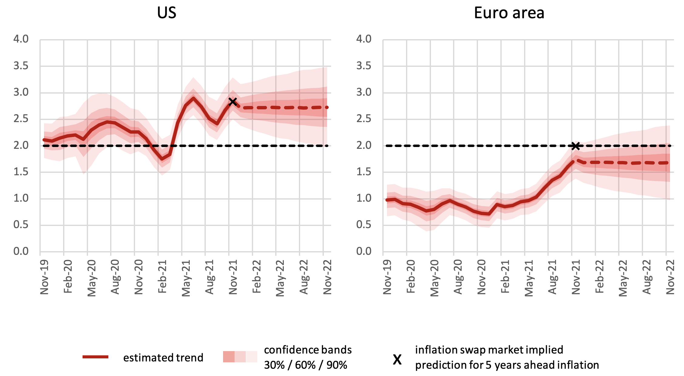
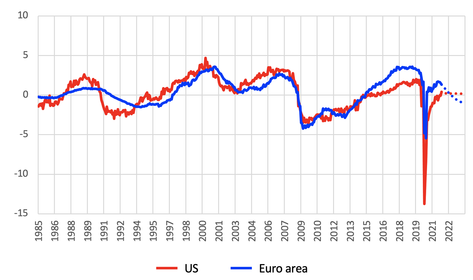
The model defines the trend as the component of inflation that is not due to cyclical components and that is reflected in professionals’ and consumers’ medium-term forecasts of inflation (see Figure 1).
Figure 1 Trend inflation in the US and euro area (%, monthly, year-on-year, not seasonally adjusted)
Sources: Authors’ computations and Now-Casting Economics Ltd.
The model suggests that, since the onset of the pandemic, the trend component of inflation has risen in both the US and the euro area by a similar amount – approximately 75 basis points. However, in the US, this rise has taken the trend well above the 2% target, whereas in the euro area it is still slightly below the target, at 1.7%.
Interestingly, for the US this is almost identical to the inflation swap market’s implied prediction for five-years-ahead inflation, while in the euro area the level identified for the trend is 25 basis points lower than the swap market’s implied prediction.
This observation gives us some comfort about the ability of our trend estimates to pin down long-term expectations. The difference between the US and the euro area also suggests that the Fed and the ECB can and should respond differently to the inflationary threat – as indeed they are doing. While in the US the inflationary pressure may have pushed the underlying inflation rate above the desired target, in the euro area it seems that inflation is still anchored below the policy target.
Oil prices and the cyclical components
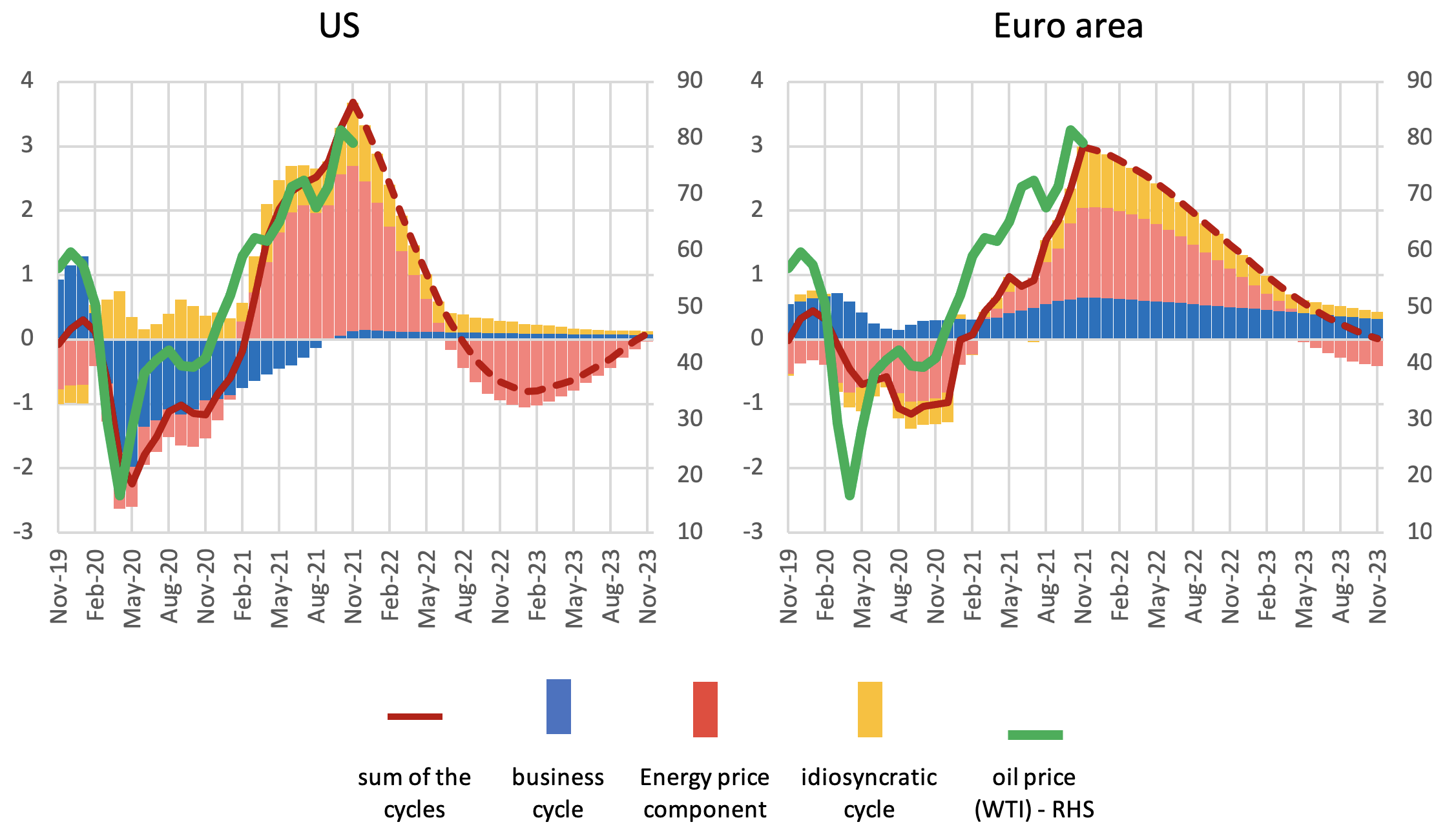
Figure 2 shows the model’s estimate of the recent and future evolution of the cyclical components of inflation: the business cycle (Phillips curve) component, the energy price component, and an idiosyncratic one. The latter may be seen as a measure of what the model cannot explain (and is indeed very small).
Figure 2 Cyclical components of inflation in the US and in the euro area
Note: The chart reports the model’s estimate of the business cycle (blue), i.e., the Phillips curve component; the energy price component (red), and an idiosyncratic component (yellow). The estimates are %, monthly, year-on-year, not seasonally adjusted.
Sources: authors’ computations and Now-Casting Economics Ltd.
The model interprets a large part of the increase in inflation over the past 18 months in both the US and the euro area as a cyclical phenomenon – but it attributes it largely to the rise in energy prices (the red bars). Consequently, the model predicts that inflation will decline in the coming months as the pressure from energy prices turns.
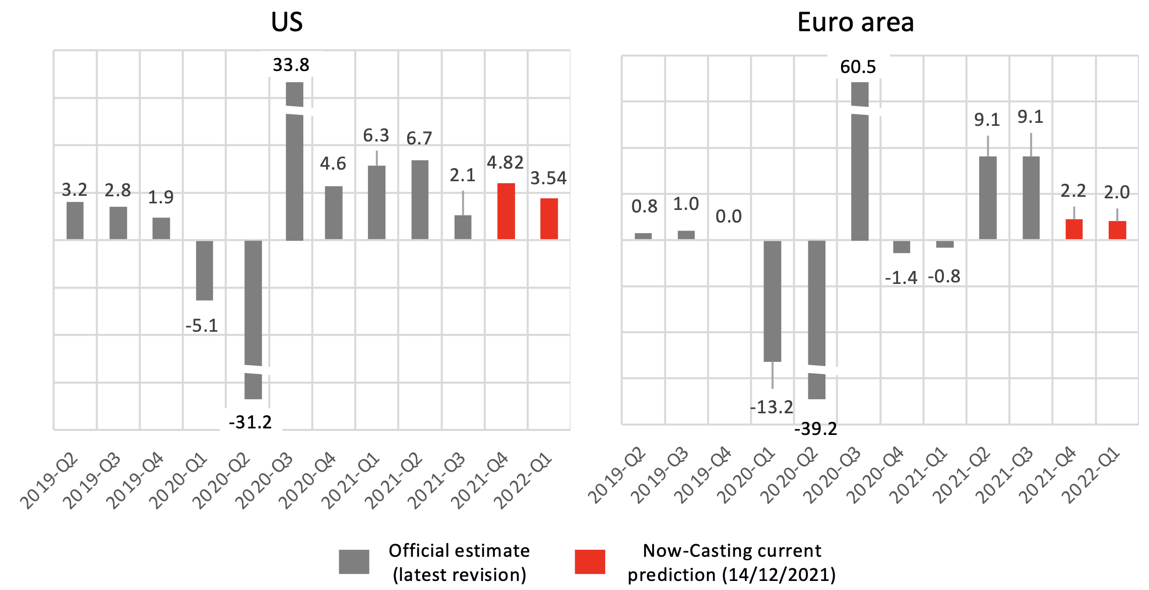
In the US, the energy price component dominates, while the real economy has little impact. By contrast, in the euro area relatively strong growth is seen to be helping to sustain the recent rise in inflation and causing its decline to be slower. This may be surprising, given that real GDP growth in the US has remained relatively strong since the post-pandemic rebound in the second half of 2020, whereas growth has been more volatile in Europe and is now apparently on a weaker path (see Figure 3). However, what matters is growth relative to trend – i.e. the output gap – and the model estimates a closing output gap with the American economy nearly back to its potential growth rate. Conversely, it estimates that the European economy has probably seen a reduction to its potential and hence it may be above trend growth (see Figure 4). Hence the impact of the Phillips curve in the US is negligible whereas in the Euro area it contributes some upward pressure on inflation until at least 2023.
Figure 3 Latest official estimates and current Now-Casting predictions of quarterly GDP growth for the US and euro area (quarter-on-quarter, %, annualized)
Sources: BEA, Eurostat and Now-Casting Economics Ltd.
Figure 4 Model’s estimates of the output gap for the US and euro area (%)
Sources: BEA, Eurostat and Now-Casting Economics Ltd.
In interpreting these results, one must be aware that there is substantial uncertainty over the size and stability of the Phillips curve but also on the estimates of trend growth.
The model view that we have just outlined is driven by two features. First, the estimates of output potential can absorb a persistent component due to shocks in the real economy – akin to hysteresis effects – and, as a consequence, the model tends to attribute less importance to cyclical variations. This is particularly true in the euro area, where the trend is revised downward, and the model is not projecting a return to the pre-pandemic trend over the next year. Second, energy prices enter the Phillips curve via mark-ups and the output gap, as in most macroeconomic models, but also have a purely expectation-driven component which is highly correlated with consumer expectations (this is in line with Coibion and Gorodnichenko 2015).
The model view of the output gap differs from official estimates for both the US and the euro area. In the US, the Congressional Budget sees a stable trend and an output gap which has been negative for more than a decade. In the euro area, again as a consequence of estimating a stable output trend, the European Commission sees a smaller output gap than our model does.
But even remaining agnostic on specific features of the cyclical decomposition, the model, by attributing the bulk of the increases in prices to a cyclical component, and in particular to energy price disturbances, orthogonal to real economic activity, appears to be consistent with past regularities. Notice that the model-based, expectation-driven oil component of the cycle is highly correlated with observed oil prices rescaled (see Figure 2), which suggests that the Phillips curve has had a minor role in cyclical inflation since 2019.
Are expectations dis-anchoring?
A pressing question is whether the model – albeit supported by historical regularities – may be missing a shift in expectations due to the effect of oil prices and the lack of a strong enough policy response.
A possible way to address this question is to examine the forecast errors made by the model in forecasting consumer expectations. Systematic negative errors would suggest a ‘bias’ in the model and possibly the drifting of inflation expectations off the target. The fact that the model has not made systematic errors in forecasting consumer inflation expectations (Figure 5) suggests no breakdown of past historical correlations and hence no strong sign of dis-anchoring (beyond that already discussed in relation to the US, where trend inflation is estimated to be 75 basis points above the target).
Figure 5 Model’s forecast errors for consumers’ expectations
Sources: BEA, Eurostat and Now-Casting Economics Ltd.
The inflation ahead
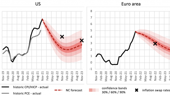
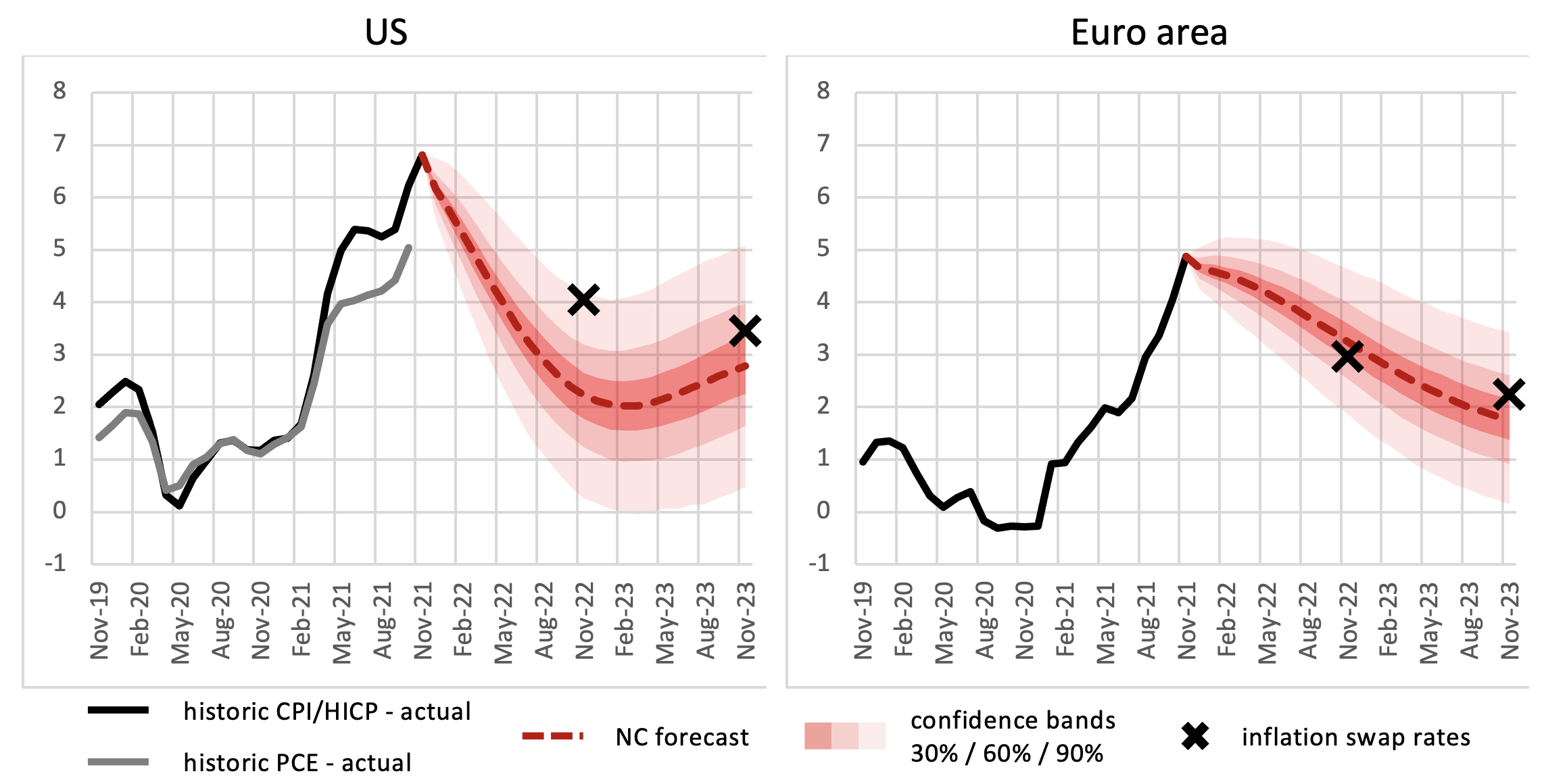
Putting together the trend and the cyclical components, we get the model’s prediction for headline inflation. In both the US and the euro area, the model predicts a cyclically dominated decline in headline inflation over the next 12 months. As we have seen, this is mainly explained by the energy cycle. Due to weaker Phillips curve pressure, the model predicts a faster decline in the US inflation rate than that for the euro area.
Figure 6 The recent path of headline CPI/HICP (monthly, year-on-year %, not seasonally adjusted) for the US and euro area, together with the model’s prediction for their paths over the next 24 months, and comparisons with the inflation swap market’s implied predictions for one- and two-years-ahead inflation.
Note: The historic path of US PCE is also shown for comparison.
Sources: BEA, Eurostat and Now-Casting Economics Ltd.
Our views seem to coincide with those of the market as reflected by inflation swap rates although the swaps predict slightly higher inflation at one year horizon for the US.
Our decomposition helps us to interpret these forecasts. It tells us that both central banks are right when they interpret current inflation as temporary, but that this view should be nuanced in different ways in the US and the euro area. In the US, as we have seen, a small but permanent increase is likely, and this implies a trend inflation rate of 2.75% in the next five years at least (assuming away unforeseeable large permanent shocks in the future).
Interpreting recent policy announcements
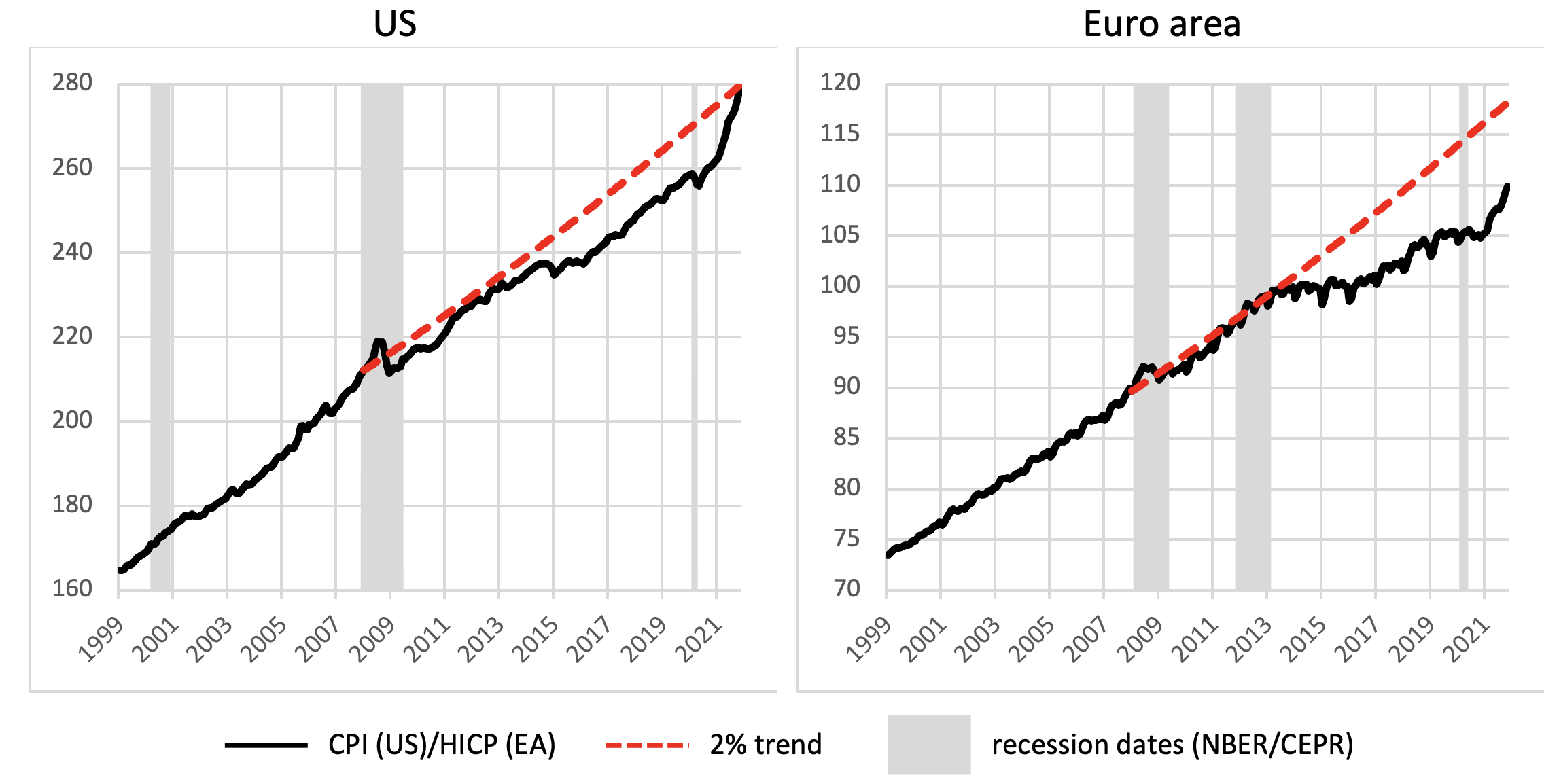
To interpret recent policy announcements, it is useful to compare the actual price level with the price level that we would have observed had inflation been at the 2% target since the recession of 2008 (in Figure 7).
Figure 7 Price levels in the US and in the euro area and the predicted price levels had the inflation target of 2% been hit since 2008
Sources: BEA, Eurostat and authors’ computations.
While in the US, the price level has returned to the level implied by the 2% target, this is not the case in the euro area. This is an additional justification for the different stance by the two central banks.
References
Coibion, O and Y Gorodnichenko (2015), "Is the Phillips Curve Alive and Well after All? Inflation Expectations and the Missing Disinflation", American Economic Journal: Macroeconomics 7(1): 197-232.
Coibion, O, Y Gorodnichenko, and S Kumar (2018), "How Do Firms Form Their Expectations? New Survey Evidence", American Economic Review 108(9): 2671-2713.
Hasenzagl, T, F Pellegrino, L Reichlin and G Ricco (2020), “A Model of the Fed's View on Inflation”, The Review of Economics and Statistics.
Hasenzagl, T, F Pellegrino, L Reichlin and G Ricco (2021), “Monitoring the Economy in Real-Time: Trends and Gaps in Real Activity and Prices”.
