Income inequality in the US has sharply increased over the last several decades. This is a well-documented fact (e.g. Gottschalk and Moffitt 1994, Katz and Autor 1999). The general public is also very interested in the issue. A recent USA TODAY/Pew Research Center poll shows that the majority of the population thinks “the economic system in the country unfairly favours the wealthy” and that the government should do “a lot to reduce the gap between the rich and everyone else.” Policymakers are aware of this as well. In his 2014 State of the Union Address, US president Barack Obama promised to tackle economic inequality “with or without Congress.” There may be several reasons for why inequality has been on the rise (for a survey, see Gordon and Dew-Becker 2008). But what about the effects of family formation on inequality?
How Americans form and dissolve families has changed dramatically since the mid-20th century.1 One of these changes has been an increase in what economists call positive assortative mating. In this context, it relates to how likely a person is to marry someone of similar educational background. Since education is an important determinant of income, these patterns of matching might have an impact on the economy's distribution of income.
Think about the following simple thought experiment. Suppose that there are only two types of people, equal in numbers, those that went to college and those who did not. Those who went to school earn $30 and those who did not earn $10. If educated men marry uneducated women and uneducated men marry educated women, then every household will earn $40 in total. So, household income is perfectly equalised. Now, imagine a world in which educated people only marry other educated people. Then, a household made up of an educated man and an educated woman will earn $60 versus the $20 earned by a household that consists of only uneducated spouses. The households at the top of the distribution would have three times the income of those at the bottom.
Obviously, the example above is a dramatic simplification of reality, but it does capture an important trend that is actually taking place in the US economy. To study its impact, we track samples of hundreds of thousands of households from the US Census Bureau for the period 1960 to 2005 (see Greenwood, Guner, Kocharkov and Santos 2014). The upshot of the analysis is that rising assortative mating together with increasing labour-force participation by married women are important in order to account for the determinants of growth in household income inequality in the US.
The rise in positive assortative mating
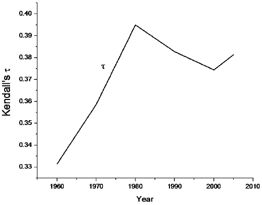
How can the degree of assortative mating be measured? Consider collapsing the levels of education into five categories: less than high school, high school, some college, college, and post college. The relationship between husband's and wife's educational levels can be measured using the Kendall's tau statistic. This statistic measures the degree of concordance between two series, here husband's and wife's educations. In a nutshell, the higher this statistic is, the higher is the degree of positive assortative mating. The changes in Kendall's tau (τ) are illustrated in Figure 1. While the series is not increasing throughout the entire period, the statistic is clearly higher in 2005 relative to 1960.
Figure 1. The rise in assortative mating
The rise in income inequality
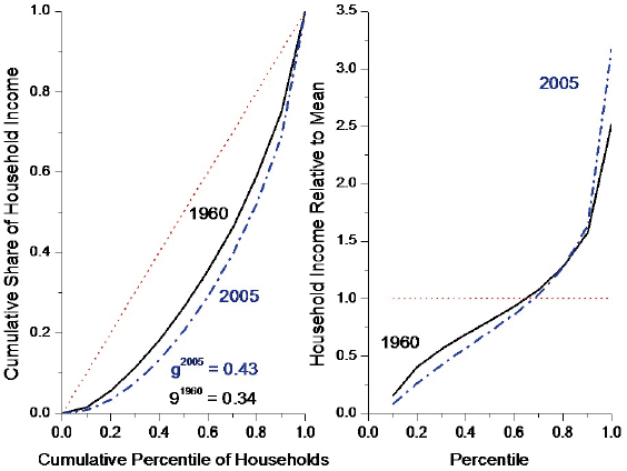
There are different ways to measure income inequality. One is through the use of Lorenz curves. The horizontal axis on a Lorenz curve plot enumerates the percentiles of households; i.e., the 20th percentile is represented by the point 0.2. The vertical axis gives share of total income in the economy that all households up to and including this percentile earn. The 45 degree line represents perfect income equality. Along the 45 degree line, households up to say the 20th percentile would earn 20% of total income. The actual Lorenz curve for the US lies below the 45 degree line. The further the Lorenz curve is from the 45 degree line, the more unequal is the income distribution. The Lorenz curves for 1960 and 2005 are pictured in the left-hand side panel of Figure 2. They show a rise in inequality. The area between the 45 degree line and Lorenz curve is a measure of income inequality. The Gini coefficient is twice this area. The Gini coefficient returns a value of zero when there is perfect income equality and has a value of one if the highest percentile earned all of the income in the economy. The Gini coefficient (g) rises from 0.34 in 1960 to 0.43 in 2005. The right-hand side panel shows the relative income for each percentile; where the rightmost percentile is the richest and the leftmost the poorest. In 1960 a household at the 10th poorest percentile earned 16% of average income. This dropped to 8% in 2005. A household in the 90th richest bracket earned 251% of average income in 1960 versus 317% in 2005. That is, incomes are more polarised in 2005.
Figure 2. Income inequality, 1960 and 2005
Assortative mating and income inequality
Both assortative mating and income inequality have increased in the data. How does marital sorting affect household income inequality? Interest in this question is not without precedence. For example, Cancian and Reed (1998) and Schwartz (2010) both conclude that an increase in assortative mating has led to a rise in income inequality. The research surveyed here, however, addresses this question using an accounting-based methodology, which is quite different from previous studies. Consider households formed by spouses with different education levels in the US Census samples. First, focus on 1960. In that year, if a woman with a less-than-high-school education married a similarly educated man, their household income would be 77% of the average household income (across all households, both single and married). If that same woman married a man with a college education, then household income would be 124% of the average. Alternatively, in 2005, if a woman with post-college education marries a man with a less-than-high-school education, their income would be 92% of average household income. This rises to 219% if her husband also has a post-college education. So, at some level, education matters for household income.
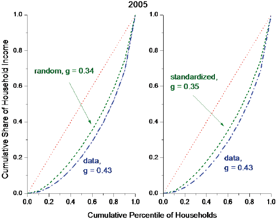
How then can one quantitatively assess this impact? One way is by again using Lorenz curves and performing a few thought experiments. Consider the following experiment. What would have happened to income inequality if matching was completely random instead of positively assortative as in the data discussed above? Moving from the observed pattern of matching to a random pattern has little discernible impact on inequality in 1960. The Gini coefficient drops only slightly from 0.34 to 0.33. Repeating the experiment for 2005 has a marked impact on income inequality, shown in the left-hand side panel of Figure 3. As can be seen, the Lorenz curve shifts closer to the perfect equality diagonal and the Gini drops from 0.43 to 0.34.
A second interesting thought experiment is to ask what would have happened to income inequality if couples in 2005 matched exactly as they did in 1960. This experiment is trickier to operationalise since people were much more educated in general in 2005 compared to 1960. This can be done by standardising the data on marital sorting.2 The results are graphed in the right-hand side panel of Figure 3. If one imposes the 1960 matching patterns for marriages on the 2005 earnings distribution for the various educational levels, the Lorenz curve shifts closer to the perfect equality diagonal, again signalling a decrease in inequality. This can also be seen by noting that the Gini coefficient drops from the original 0.43 to 0.35 in the experiment. So, if people matched in 2005 according to the standardised mating pattern observed in 1960, which showed less positive assortative mating, then income inequality would drop because household income would be more diversified across husband and wife.
Figure 3. The effects of assortative mating on inequality
References
Cancian, Maria and Deborah Reed (1998), “Assessing the Effects of Wives' Earnings on Family Income Inequality.” The Review of Economics and Statistics, vol. 80 (1): 73-79.
Fernandez, Raquel and Richard Rogerson (2001), “Sorting and Long-Run Inequality”, Quarterly Journal of Economics, vol. 116 (4): 1305-1341.
Gordon, Robert J and Ian Dew-Becker (2008), “Controversies about the Rise of American Inequality: A Survey.” NBER Working Paper 13982.
Gottschalk, Peter and Robert Moffitt. (1994), “The Growth of Earnings Instability in the US Labor Market”, Brookings Papers on Economic Activity, vol. 25 (2): 217-272.
Greenwood, Jeremy, Nezih Guner, Georgi Kocharkov and Cezar Santos (2014), “Marry Your Like: Assortative Mating and Income Inequality”, NBER Working Paper 19829.
Greenwood, Jeremy, Nezih Guner, Georgi Kocharkov and Cezar Santos (2012), “Technology and the Changing Family: A Unified Model of Marriage, Divorce, Educational Attainment and Married Female Labor Force Participation”, NBER Working Paper 17735.
Katz, Lawrence and David Autor (1999), “Changes in the Wage Structure and Earnings Inequality”, In: O Ashenfelter and D Card (ed.), Handbook of Labor Economics, ed. 1, vol. 3, ch. 26, 1463-1555, Elsevier.
Mosteller, Frederick. (1968), “Association and Estimation in Contingency Tables”, Journal of the American Statistical Association 63 (321): 1-28.
Schwartz, Christine (2010), “Earnings Inequality and the Changing Association between Spouses' Earnings.” American Journal of Sociology, vol. 115 (5): 1524-1557.
1 For an economic model that incorporates many of these changes, see Fernandez and Rogerson (2001) and Greenwood et al. (2012).
2 The procedure followed is outlined in Mosteller (1968). See Greenwood, Guner, Kocharkov and Santos (2014) for a discussion on how the procedure can be applied to the present question.


