Housing is fundamental to the economy, but for too long has remained outside mainstream of academic research. For most households in advanced economies, housing is the largest component of wealth. Since WWII, lending backed by housing collateral has become the dominant share of debt issued by the financial sector (Jordà et al. 2014, 2016). Residential investment, subject to major cyclical swings, is a large component of overall investment. For the US, where housing collateral is strongly linked with consumer spending, Leamer (2015) argues that the housing cycle is the business cycle.1 Our survey paper on housing market dynamics (Duca et al. 2021) includes an analysis of the role of housing in the financial accelerator that drove the Global Financial Crisis.
Given their depth and complexity, the interactions between housing and the wider economy affect many intertwined aspects of public policy analysed by the OECD (2021). For example, housing has important implications for job matching and labour markets. Mobility-restricting policies such as high transaction taxes, severe land-use restrictions, or ‘locking’ tenants into non-transferable social housing may trap workers in unemployment or low-productivity jobs. Restrictions, such as those on building height, urban growth boundaries, and other types of zoning can make housing less affordable and promote urban sprawl, with consequences for air pollution and energy use that ultimately conflict with global climate goals.
Here, we draw five major lessons from our survey paper on the vast international literature on housing market dynamics.
The efficient market rational expectations paradigm does not fit housing
Heterogeneity, trading and search costs, transaction delays, asymmetric information, and credit constraints are rife in housing markets and account for the drawn-out adjustment of prices to shifts in fundamentals.2 The time it takes housing supply to adjust helps explain the longer-term volatility of house prices – the result of the interplay between short- to medium-run bubble builder and longer-term bubble burster dynamics (Abraham and Hendershott 1996). This limits the potential usefulness of including simple housing sub-models in micro-founded representative agent dynamic stochastic general equilibrium (or DGSE) models, such as that of Iacoviello and Neri (2010). Housing economists have long known that house price changes are positively correlated, and that past information on fundamentals forecasts excess returns.3 Among recent studies documenting extrapolative house price expectations in the US, Barberis et al. (2018) show how such expectations by some investors can generate asset price bubbles.4 These are consistent with calibrations from theoretical models with expectations prone to momentum (Glaeser and Nathanson 2017, Piazzesi and Schneider 2016). Extrapolative expectations or other forms of non-fully rational, backward-looking expectations (Gennaioli and Shleifer 2018) play a key role in most empirically plausible narratives of housing booms and busts, including the US subprime boom and bust of the 2000s.5
Simple house price-to-rent arbitrage models are misleading
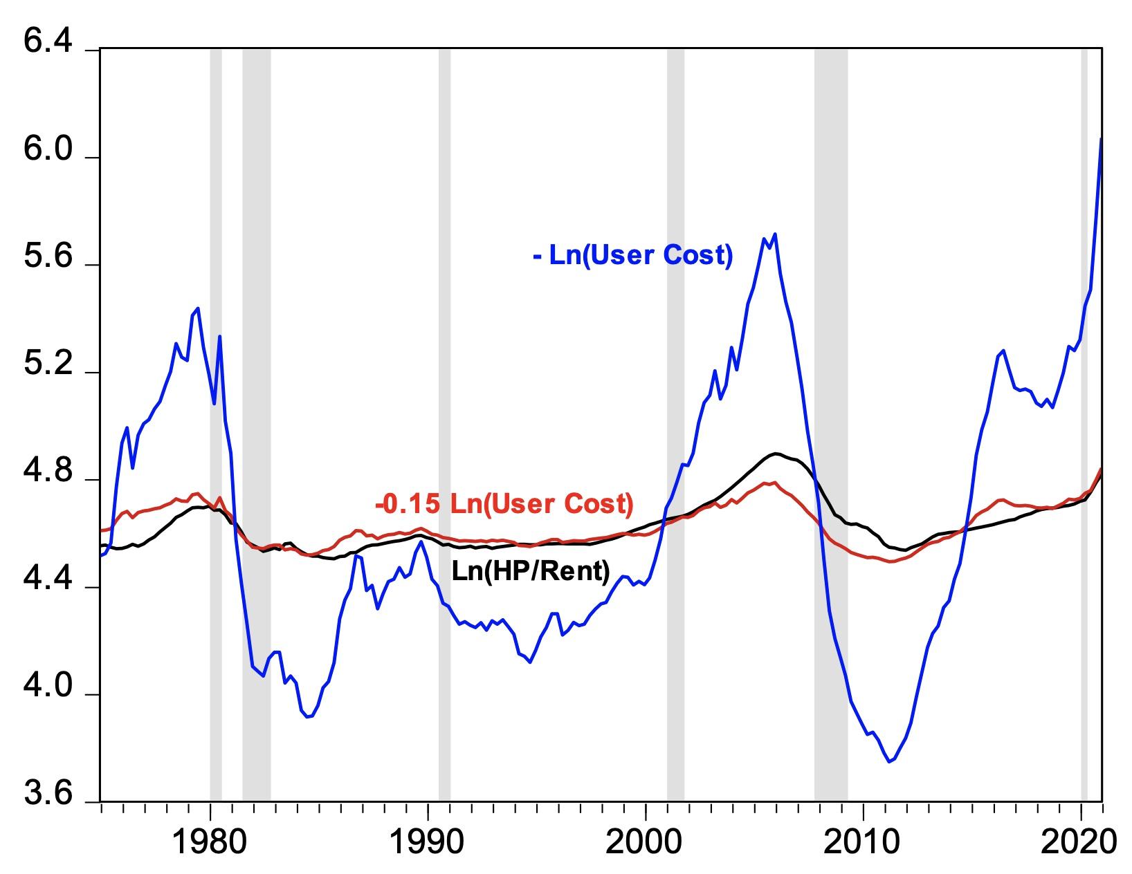
The simple arbitrage theory – in which the value of a home is merely the discounted present value of future rents – is inappropriate for explaining variation in house prices. The theory is based on perfect arbitrage between rents and house prices, which, under restrictive assumptions, implies that the price-to-rent ratio moves one-for-one with the inverted user cost of housing. This implies that the log price-to-rent ratio equals minus log user cost. The user cost is typically tracked by an after-tax nominal mortgage rate minus a proxy for the expected rate of house price appreciation. Using annualised house price appreciation over the previous four years as an expectations proxy, the user cost (taking into account transactions costs, tax-deductible interest and property taxes and home-owners insurance) grossly exaggerates swings in the US house price-to-rent ratio (Figure 1) when the scales impose a unitary elasticity. But a scaling of 0.15 fits long-run fluctuations in the price-to-rent ratio far better.6
The simple theory is inappropriate for several reasons. One is that owner-occupied properties, which dominate US house price indices, often have more land per occupant than rentals, implying that these property types are far from perfect substitutes (Glaeser and Gyourko 2009). In practice, rents are far ‘stickier’ and less cyclical than house prices. This is so partly because they are less sensitive to highly cyclical land prices. Other factors include differences in the characteristics of renters, and the unobserved costs and benefits of owning versus renting. Large transaction costs, risk aversion, and the volatility of house prices make it hard to arbitrage between renting and buying.
Figure 1 The US house price-to-rent ratio violates the unit user cost elasticity of the simple arbitrage model
Sources: FHFA, Freddie Mac, BLS, BEA, Federal Reserve Board.
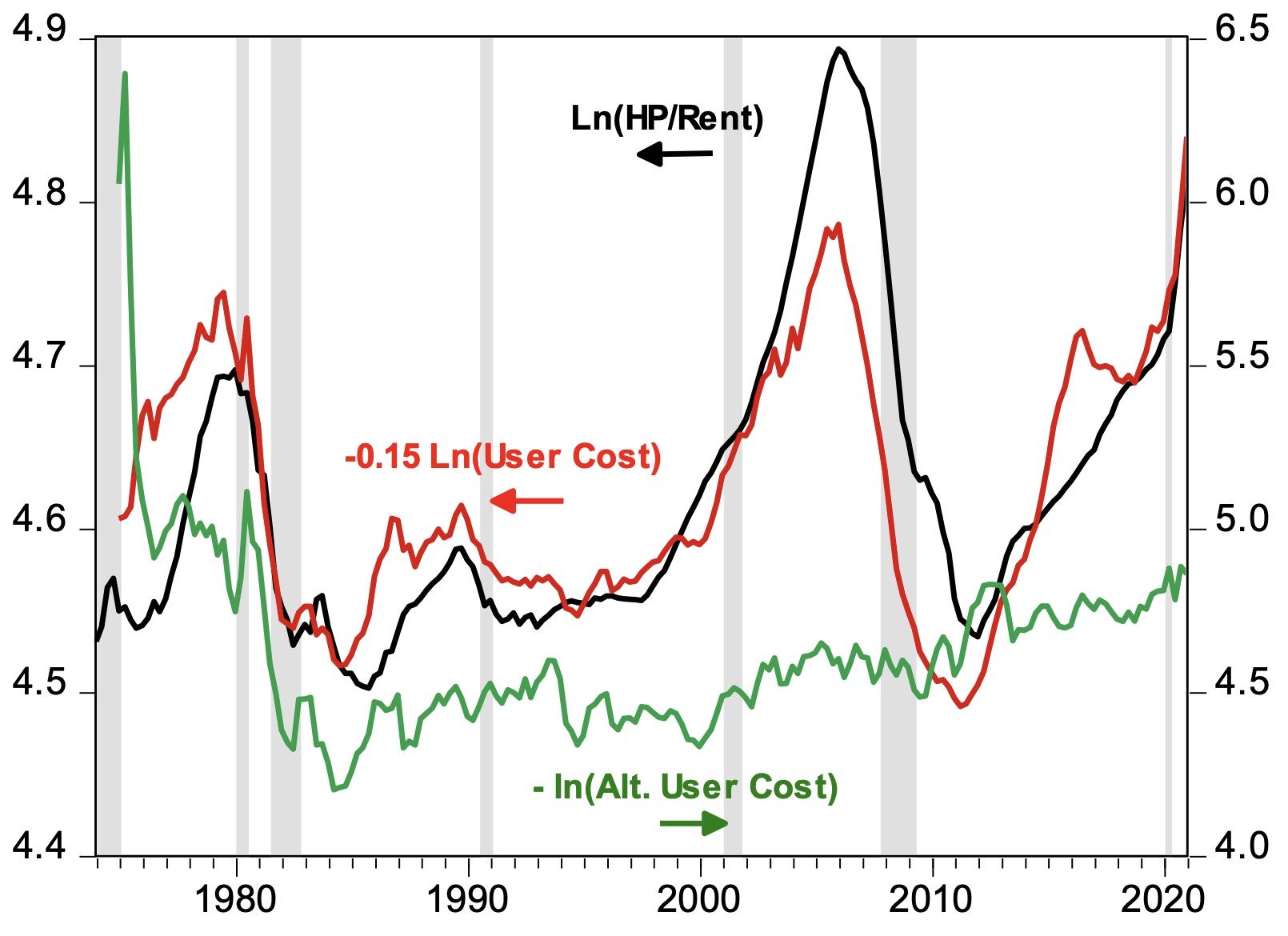
Some empirical studies of house price dynamics use a real mortgage interest rate as a proxy for user cost. Figure 2 illustrates such a user cost proxy with similar tax and transactions costs adjustments, representing expected house price appreciation by annual consumer price inflation plus the annual appreciation of real house prices averaged over 50 years (1⅓%). Figure 2 makes it clear that this measure of user costs is inferior to basing expected appreciation on the average of the previous four-year house price appreciation.
The second key failure of the simple rent arbitrage relationship stems from its neglect of credit constraints. With a credit constraint, the efficiency condition linking house prices and rents needs to be augmented by the shadow price of the credit constraint (Dougherty and Van Order 1982, Henderson and Ioannides 1983, Meen 1990). Since many lenders use debt service-to-income ratios to allocate mortgage credit, falls in nominal interest rates, unlikely to increase rents, expand credit availability and so increase house prices (Kearl 1979).
Figure 2 Alternative user cost measure does not line up with hp/rent ratio
Note: Alternative user cost measure uses real mortgage rate and long-run average annual real house price appreciation.
Sources: See Figure 1.
Shifts in credit conditions are a key driver of house prices
Confirming the importance of credit conditions, Duca et al. (2016) find that the log of the US house price-to-rent ratio is not cointegrated with the log user cost over 1983-2013. But adding the (highly significant) loan-to-value ratio for first-time home buyers – an important marginal group of buyers, with many facing credit constraints – as a proxy for the shadow price on the credit constraint achieves cointegration.7 This is consistent with a burgeoning post-crisis literature, such as Mian and Sufi (2018). This literature highlights the need for sound financial regulation (Cesa-Bianchi and Rebucci 2013). To track the credit channel and monetary transmission in econometric policy models, future generations of these models will need to incorporate insights from these research findings.
Differences in land supply responses explain much of observed spatial variation
The second major approach to modelling housing house prices – the inverted demand approach – implies that valuation cycles are driven by several factors. These include user costs, income, credit constraints, and supply conditions. Here, the demand function is inverted to obtain house prices as a function of the given housing stock and the demand drivers.8 For a fuller model, a second equation for residential investment is needed to explain variations in the housing stock. The responsiveness of such investment to house prices varies with the severity of land supply constraints. But implementing this approach can be hampered by the unavailability of good housing stock data. The price-to-rent approach also needs good data, but on market rents. When modified to allow for credit constraints, non-rational house price expectations, and imperfect substitution between multi-family and detached owner-occupied housing, this approach also needs a second equation, namely for rents. Such an equation needs to take into account the supply-demand balance in housing markets and should not assume that rents are exogenous to housing markets.9
Across US metros, house price bubbles are more frequent and larger in more supply inelastic areas (Glaeser et al. 2008).10 Glaeser et al. (2008) and other studies find that differences in supply elasticities arise mainly from variations in the availability of land, rather than in construction costs. Using Saiz’s (2010) supply elasticity estimates (and work by Oikarinen et al. (2018) for cross-sectional dependence), it is found that the income elasticity of house prices is higher, and that the duration and size of bubbles is larger in metros with less elastic land supply.
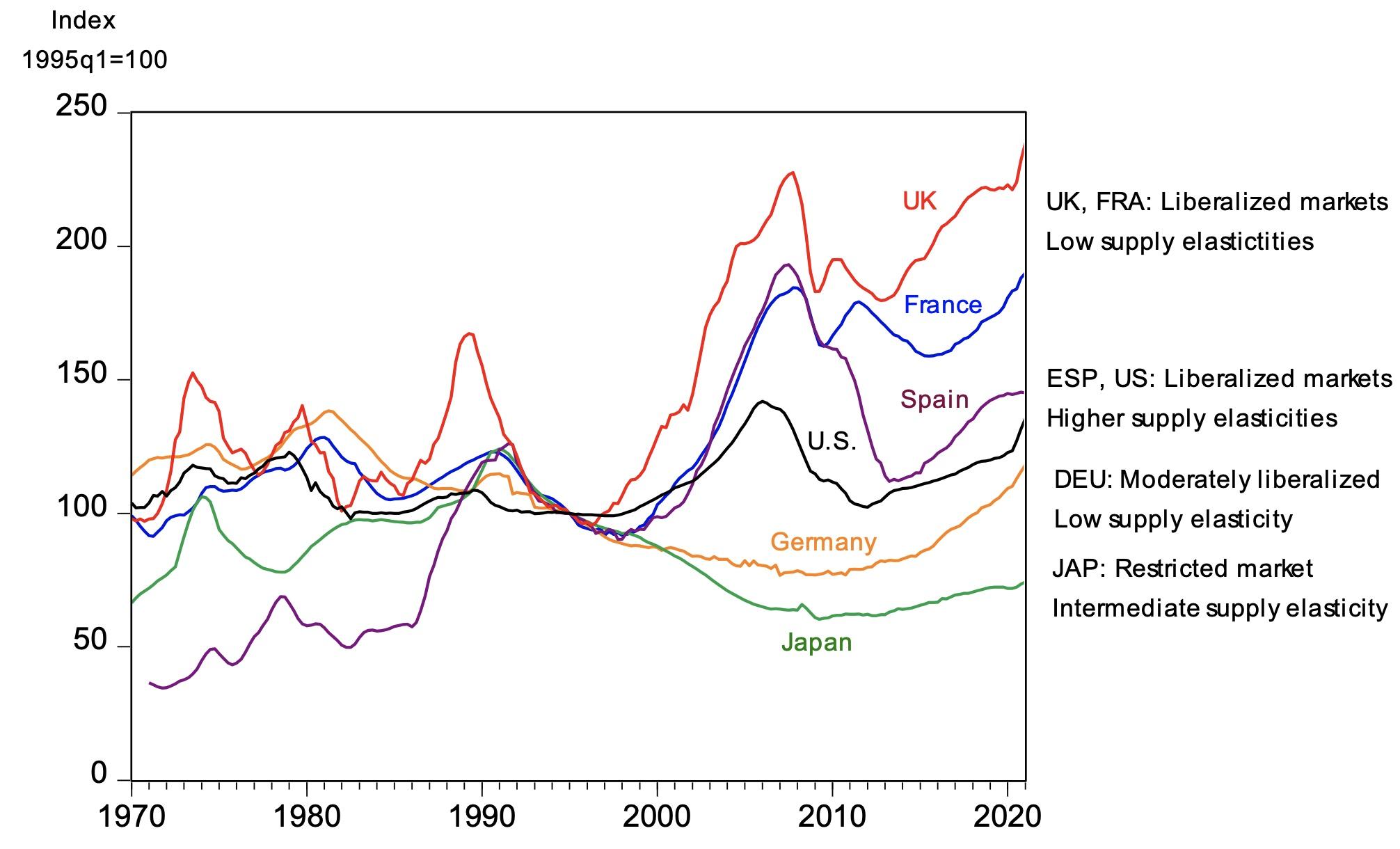
Figure 3 House price-to-rent ratios vary across countries and over time
Source: OECD
At the national level, differences in credit availability (Cerutti et al. 2017) and in housing supply are also linked to house prices. Among the six nations in Figure 3, Cavalleri, et al. (2019) rank the US as having the most price elastic supply of housing,11 with lower elasticities in France, Germany, and the UK. Over the past half century, the UK saw the strongest house price-to-rent rise stemming from strong demand (liberalised credit plus strong income and population growth) pushing up against inelastic supply (Hilber and Vermeulen 2016). France, with partly-liberalised markets, had the next highest price rise, with less elastic supply to limit prices than Spain (which had the third highest rise) and then the US. At the bottom are Germany and Japan, where credit was not liberalised and population growth was low (though valuations have risen in Germany, which has benefitted from the euro area recovery from the Global Financial Crisis).
Why house prices didn’t collapse in the pandemic
More research is needed to better integrate expectations formation and heterogeneity into models, to account for cross-sectional dependence and time variation, and to address important gaps in data. Nevertheless, the recent literature has lessons for the future and for the impact of the pandemic on housing markets.
House prices behaved differently in the Covid-19 recession than in prior downturns for several reasons. The initial shocks differed, the financial system was better capitalised, and most households were not overly indebted (especially in contrast to the US Great Recession). There was a very quick and broad set of economic policy responses. Relevant for housing were the (a) use of unconventional and conventional monetary policy to lower long-term interest rates; (b) imposition of moratoria on foreclosures/home repossessions and renter evictions; (c) aggressive modification of mortgages to prevent defaults; and (d) large transfer payments to households, the unemployed and furloughed workers coupled with significant credit support to firms, and (in some countries) employment subsidies that buttressed household income. These actions prevented a long recession and a financial crisis.
Consequently, and in contrast to the Global Financial Crisis, house prices rose sharply in some countries, such as the US, the UK, France, and Germany (see Figure 3).12 Lower interest rates and a Covid-related relative rise in the demand for detached housing (and space in general) initially boosted house prices.13 On the supply side, lockdowns, pandemic related supply chain disruptions, and labour shortages reduced the supply of new housing. The effects on house prices via the user cost were plausibly amplified by households’ tendency to form extrapolative expectations of house prices. But the substantial re-regulation of mortgage lending in advanced countries (such as the Dodd-Frank Act in the US) has likely limited the role for shifts in credit standards in fuelling the recent surge in prices.
Conclusion
Our careful review of recent research cautions against focusing too much on the role of real interest rates driving house price booms and busts to the exclusion of other key factors discussed above.14 In this regard, looking beyond the pandemic, a key lesson is that housing policy needs to be holistic to address the lack of housing affordability that many nations and regions face (see OECD 2021).
Authors’ note: The views expressed are those of the authors and do not necessarily reflect the views of the Federal Reserve Bank of Dallas or the Federal Reserve System.
References
Aastveit, K, B Albuquerque and A K Anundsen (2020), “The Declining Elasticity of US Housing Supply”, VoxEU.org, 25 February.
Abraham, J M and P H Hendershott (1996), “Bubbles in Metropolitan Housing Markets”, Journal of Housing Research 7(2): 191-207.
Anundsen, A K and C Heebøll (2016), “Supply Restrictions, Subprime Lending and Regional US House Prices”, Journal of Housing Economics 31(1): 54-72.
Armona, L, A Fuester and B Zafar (2019), “Home Price Expectations and Behaviour: Evidence from a Randomized Information Experiment”, Review of Economic Studies 86(4): 1371-1410.
Barberis, N, R Greenwood, L Jin and A Shleifer (2018), “Extrapolations and Bubbles”, Journal of Financial Economics 129(2): 203-227.
Capozza, D R and P J Seguin (1996), “Expectations, Efficiency, and Euphoria in the Housing Market”, Regional Science and Urban Economics 26(3–4): 369-386.
Case K E and R J Shiller (1989), “The Efficiency of the Market for Single-Family Homes”, American Economic Review 79(1): 125-137.
Case, K E and R J Shiller (1990), “Forecasting Prices and Excess Returns in the Housing Market”, Real Estate Economics 18(3): 253-273.
Case, K E, R J Shiller and A K Thompson (2012), “What Have They Been Thinking? Homebuyer Behavior in Hot and Cold Markets”, Brookings Papers on Economic Activity 43(2): 265-298.
Cavalleri, M C, B Cournède and E Özsöğüt. (2019), “How Responsive are Housing Markets in the OECD? National Level Estimates”, OECD Working Paper 1590.
Cerutti, E, J Dagher and G Dell’Ariccia (2017), “Housing Finance and Real Estate Booms: A Cross-Country Perspective”, Journal of Housing Economics 38: 1-13.
Cesa-Bianchi, A and A Rebucci (2013), “Is the Federal Reserve Breeding the Next Financial Crisis?”, VoxEU.org, 11 April.
Clayton, J (1997), “Are Housing Price Cycles Driven by Irrational Expectations?”, Journal of Real Estate Finance and Economics 14 (3): 341-363.
DeFusco, A A, C G Nathanson and E Zwick (2017), “Speculative Dynamics of Prices and Volume”, NBER working paper 23449.
De Stefani, A (2020), “House Price History, Biased Expectations and Credit Cycles”, Real Estate Economics, June: 1– 29.
Dougherty, A and R Van Order (1982), “Inflation, Housing Costs, and the Consumer Price Index”, American Economic Review 72(1): 154-164.
Duca, J V, M Hoesli and J Montezuma (forthcoming), “The Resilience and Realignment of House Prices in the Era of COVID-19”, Journal of European Real Estate Research.
Duca, J V, J Muellbauer and A Murphy (2016), “How Mortgage Finance Reform Could Affect Housing”, American Economic Review 106(5): 620-624.
Duca, J V, J Muellbauer and A Murphy (2021), “What Drives House Price Cycles? International Experience and Policy Issues”, Journal of Economic Literature 59(3): 773-864.
Gennaioli, N and A Shleifer (2018), A Crisis of Beliefs: Investor Psychology and Financial Fragility, Princeton, NJ: Princeton University Press.
Glaeser, E L and J Gyourko (2009), “Arbitrage in Housing Markets”, in E L Glaeser and J M Quigley (eds) Housing Markets and the Economy: Risk, Regulation, and Policy, Cambridge, MA: Lincoln Institute of Land Policy.
Glaeser, E L (2013), “A Nation of Gamblers: Real Estate Speculation and American History”, American Economic Review 103(3): 1-42.
Glaeser, E L, J Gyourko and A Saiz (2008), “Housing Supply and Housing Bubbles”, Journal of Urban Economics 64 (2): 198–217.
Glaeser, E L and C G Nathanson (2017), “An Extrapolative Model of House Price Dynamics,” Journal of Financial Economics 126(1): 147-170.
Gupta, A, J Peeters, V Mittal and S Van Nieuwerburgh (2021), “Flattening the Curve: Pandemic-Induced Revaluation of Urban Real Estate”, VoxEU.org, 11 February.
Hamilton, B W and R M Schwab (1985), “Expected Appreciation in Urban Housing Markets”, Journal of Urban Economics 18(1): 103-118.
Henderson, J V and Y Ioannides (1983), “A Model of Housing Tenure Choice”, American Economic Review 73(1): 98-113.
Hilber, C and W Vermeulen (2016), “Regulation is to Blame for England’s Surging House Prices”, VoxEU.org, 10 April.
Iacoviello, M and S Neri (2010), “Housing Market Spillovers: Evidence from an Estimated DSGE Model”, American Economic Journal: Macroeconomics 2(2): 125-164.
IMF, Financial Stability Board and Bank for International Settlements (2016), Elements of Effective Macroprudential Policies: Lessons from International Experience, Washington, DC: IMF.
Jordà, Ò, M Schularick and A M Taylor (2014), “The Great Mortgaging”, VoxEU.org, 12 October.
Jordà, Ò, M Schularick and A M Taylor (2016. “The Great Mortgaging: Housing Finance, Crises and Business Cycles”, Economic Policy 31(85): 107-152.
Leamer, E E (2015), “Housing Really Is the Business Cycle: What Survives the Lessons of 2008– 09?”, Journal of Money, Credit and Banking 47(S1): 43-50.
Meen G P (1990), “The Removal of Mortgage Market Constraints and the Implications for Econometric Modelling of UK House Prices”, Oxford Bulletin of Economics and Statistics 52(1): 1-23.
Meese, R and N Wallace (1994), “Testing the Present Value Relation for Housing Prices: Should I Leave My House in San Francisco?”, Journal of Urban Economics 35(3): 245-266.
Mian, A R and A Sufi (2011), “House Prices, Home Equity–Based Borrowing, and the U.S. Household Leverage Crisis”, American Economic Review 101(5): 2132-2156.
Mian, A R and A Sufi (2018), “Credit Supply and Housing Speculation”, VoxEU.org, 19 August.
Mian, A R, A Sufi and E Verner (2017), “Household Debt and Business Cycles Worldwide”, Quarterly Journal of Economics 132(4): 1755-1817.
Miles, D, and V Monro (2019), “UK House Prices and Three Decades of Decline in the Risk Free Real Interest Rate”, Bank of England Staff Working Paper 837.
Muellbauer, J (2008), “Housing Wealth and Consumer Spending”, VoxEU.org, 20 July.
Niu, G and A van Soest (2014), “House Price Expectations”, IZA Discussion Paper 8536.
OECD (2021), Brick by Brick: Building Better Housing Policies, Paris: OECD.
Oikarinen, E, S C Bourassa, M Hoesli, and J Engblom (2018), “U.S. Metropolitan House Price Dynamics”, Journal of Urban Economics 64: 54-69.
Piazzesi, M and M Schneider (2016), “Housing and Macroeconomics”, in J B Taylor and H Uhlig (eds), Handbook of Macroeconomics, Amsterdam: North-Holland.
Poterba, J M (1991), “House Price Dynamics: The Role of Tax Policy and Demography”, Brookings Papers on Economic Activity 22(2): 143-203.
Ramani, A and N Bloom (2021), “The Doughnut Effect of COVID-19 on Cities”, VoxEU.org, 28 January.
Saiz, A (2010), “The Geographic Determinants of Housing Supply”, Quarterly Journal of Economics 125(3): 1253-1296.
Endnotes
1 Mian and Sufi (2011) emphasize home equity borrowing and the leverage cycle in the US. A similarly strong link in the UK led Muellbauer (2008) to explain why a major recession was imminent.
2 In practice, house prices are far from the ‘jump variable’ specified in rational expectations models as empirical models of reactions of house prices to fundamentals show speeds of adjustment rarely above 15% per quarter. However, in some circumstances speculative frenzies can occur.
3 Older papers emphasizing this point include Hamilton and Schwab (1985), Case and Shiller (1989, 1990), Poterba (1991) and Meese and Wallace (1994), Capozza and Seguin (1996) and Clayton (1997).
4 See also Niu and van Soest (2014), Armona, Fuester and Zafar (2016), Defusco, Nathanson and Zwick (2017) and De Stefani (2020).
5 See Case, Shiller and Thompson 2012, Glaeser 2013, Glaeser and Nathanson 2017, and Defusco, Nathanson and Zwick 2017.
6 In other words, we replace -1 log user cost by -0.15 log user cost in the plot against the log house price-to-rent ratio, see Duca, Muellbauer and Murphy (2016).
7 Cointegration implies that, in the long run, the log house price-to-rent ratio cannot drift far away from the value implied by the linear combination of log user cost and the median first-time buyer LTV. In the current instance, shifts in the median LTV also precede shifts in user cost, emphasizing its causal role.
8 This approach follows the demand for durable goods in consumer economics, in which the demand for housing depends on the price, and on user cost, current and expected income, demography, and financial wealth components. The demand function is inverted to obtain house prices as a function of the given housing stock and the demand drivers.
9 Econometric modelling of rents is an under-researched area of economics.
10 More recent US evidence suggests that larger price rises in such areas induced construction swings in the subprime boom and bust that did not differ much from those in more price elastic areas (Anundsen and Heebol, 2016).
11 Though Aastveit, Albuquerque and Anundsen 2020 argue that elasticities in the US have declined.
12 In contrast, valuations were stagnant in Japan, where valuations have been dampened by continued sharp declines in population, and in Spain, where household income was less sustained by remote working and where house prices were dampened by COVID-related declines in tourism and the demand for second homes by foreign nationals, see Duca, Hoesli and Montezuma 2021.
13 See Gupta et al. (2021) for evidence on the flattening of the urban house price and rent gradients between central and more peripheral locations. Ramani and Bloom (2021) point out the pandemic’s “donut effect” on the relative prices of suburban versus urban house prices.
14 We differ with Miles and Munro 2019, who, using the simple rent-arbitrage relationship, claim that the 1985–2018 rise in UK house prices relative to income is explained by the fall in the risk-free interest rate and had little to do with supply constraints.


