The question “When did Argentina lose its mojo?”, a paraphrasis of a famous Latin American novel, defines a recurrent debate about the growth underperformance of Argentina.
A country recognised as a class in itself, Argentina evolved from “relative wealth to relative poverty” (Pritchett 1997, De Long 1988); it is the archetypal example of economic divergence.
The literature has often addressed the question from a descriptive perspective: visual inspection of the comparative evolution of per capita income series relative to developed economies. In a new paper (Katz and Levy Yeyati 2024), we propose a metric to characterise and date Argentina’s secular divergence.
We use as our benchmark a group of economies (Austria, Australia, Belgium, Canada, Denmark, France, Germany, and the Netherlands) that, adjusting for purchasing power parity (PPP), have similar per capita GDP (within a 50% interval centred in Argentina’s per capita income) at the beginning of the period of analysis (based on data reliability, we chose the year 1900 as our starting point and use the centred ten-year average to compute per capita income).
We HP-filter the GDP series to focus on trends (and abstract from one-off events or cyclical movements), compute each country’s per capita income gap with Argentina, and average the gaps. We do the same for population and GDP.
The basic narrative
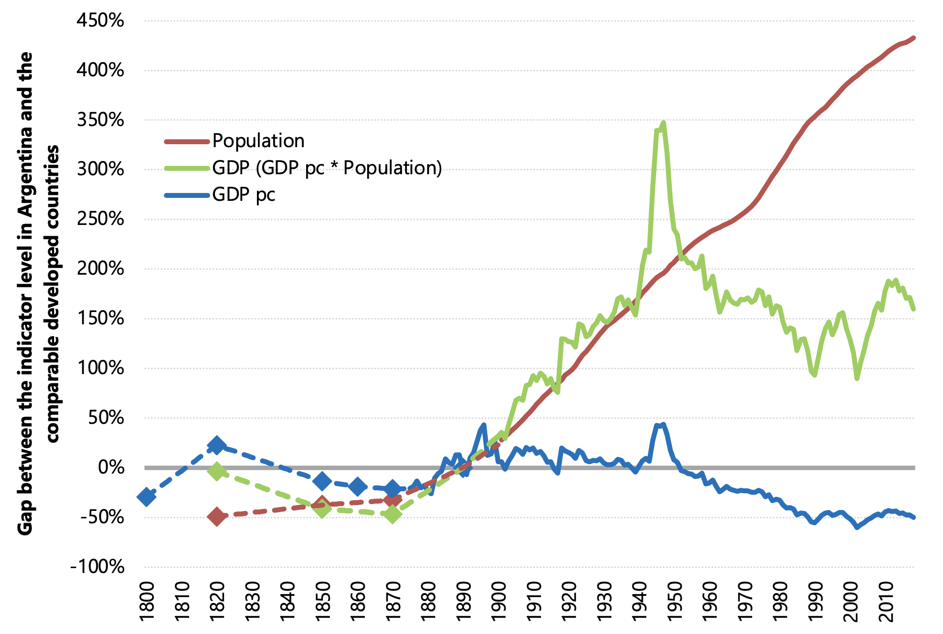
Figure 1 shows the three series. Up to 1950, the decline coincides with a strong relative growth of both real GDP and population (the stronger performance of the latter explains the relative decline in per capita terms). By contrast, the accelerated economic divergence of the second half cannot be attributed primarily to demographic factors: not only is there a more subdued relative increase in population; unlike in the previous phase, there is also a marked relative decline in GDP.
Figure 1 Relative evolution of total GDP, population, and per capita GDP (1890=100)
Source: Own elaboration based on Maddison Project Database (2020).
Note: The original series by country are smoothed using an HP filter with a start date of 1880 and converted to 1890=100 base. We calculate the gap relative to each of the benchmark countries, from which we obtain the average gap reported in the figure. Dashed lines indicate interpolated data.
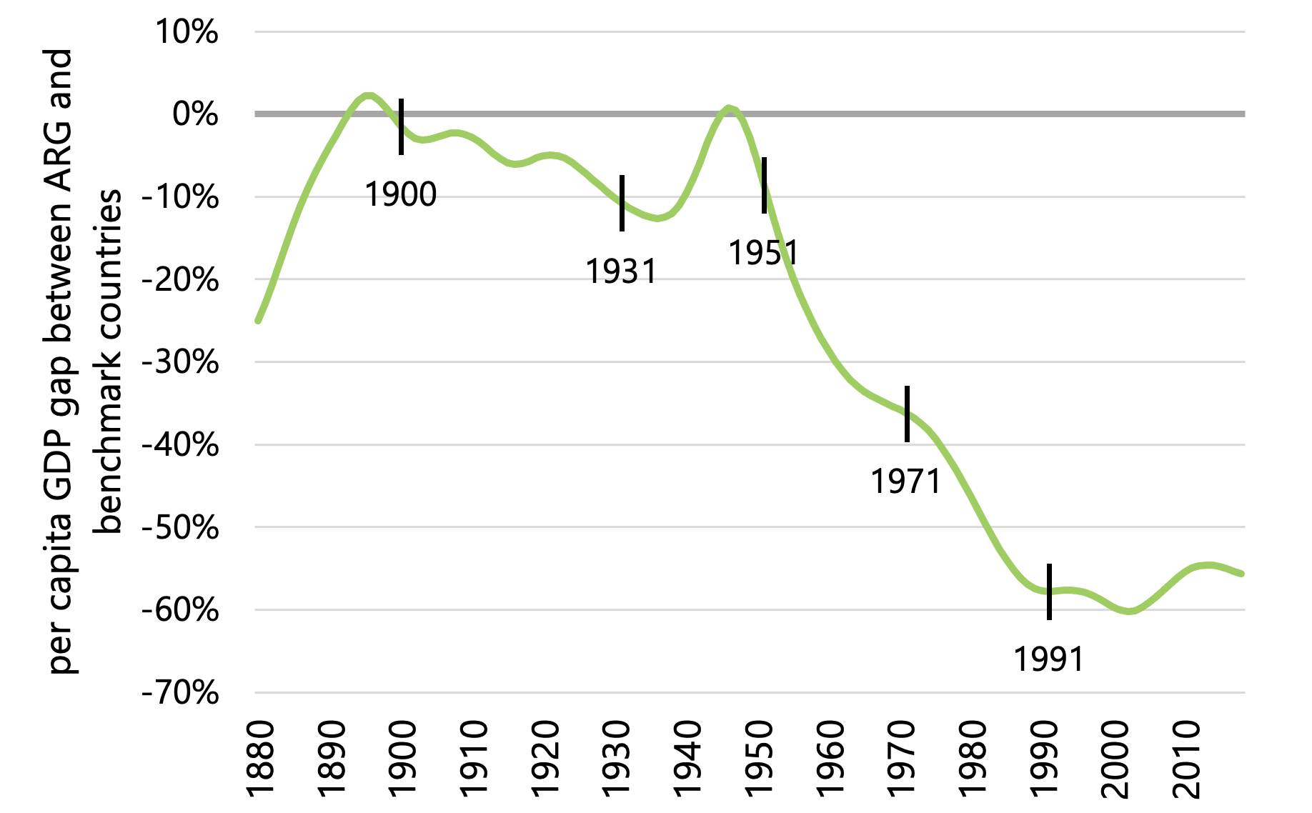
Figure 2 presents the inflection points identified using Bai and Perron’s (1998) Global L versus None Multiple Breakpoint test.
The break points, indicated with vertical lines, are mostly consistent with the anecdotal story that emerges from Figure 2: a mild divergence in the period 1900–1930s, a brief recovery during WWII, an accelerated decline from 1950 onwards (with a brief a pause in the mid-1960s), and a ‘plateau’ starting in the 1990s.
Figure 2 Per capita GDP relative to benchmark countries (HP-filtered trends)
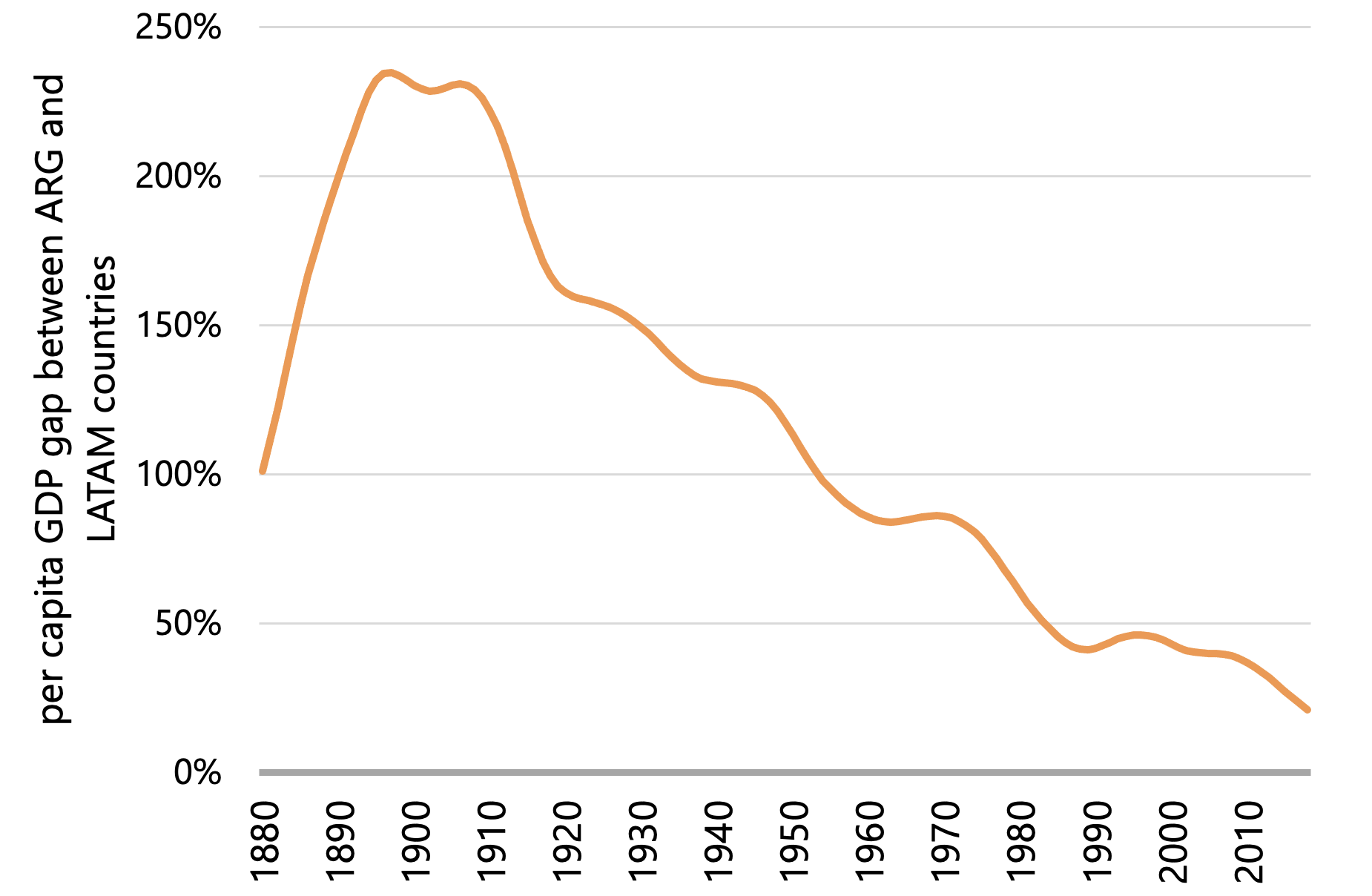
We replicate the previous exercise for a representative group of Latin American countries (Brazil, Chile, Colombia, Mexico, Peru, and Uruguay) to compare Argentina with economies that have similar factor endowments and geographical locations, and to document the reverse phenomenon: Argentina’s convergence (from above) to neighbouring economies materialises not through an upward convergence of the latter, but through the relative decline of the former (the Latin American sample does not exhibit a long-run convergence to the developed economies in the benchmark). Figures 3 and 4 illustrate these points.
Figure 3 Per capita GDP relative to Latin American countries (HP-filtered trends)
Source: Own elaboration based on Maddison Project Database (2020).
Note: The Mexico series incorporated in the LATAM average includes linear interpolations in the interval 1880–1900 to complete missing data.
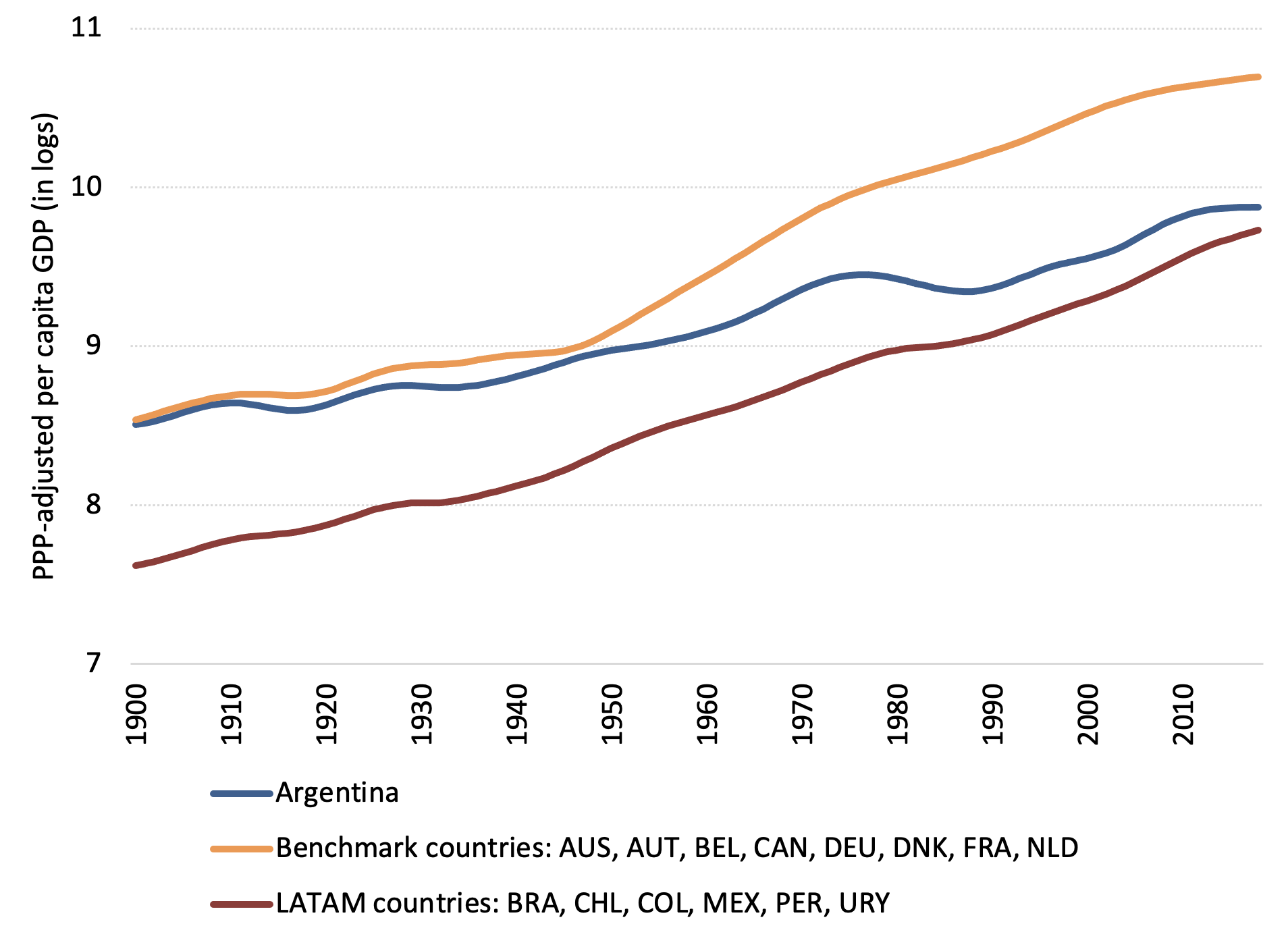
Figure 4 illustrates both the divergence of Argentina with respect to the benchmark and the convergence from above to its neighbours. The GDP series are presented in levels (logs) for the sake of visual comparison. As noted, Latin American (LATAM) countries do not exhibit any visible convergence to the income levels of the most advanced economies in the benchmark: it is Argentina that lags behind, distancing itself from the advanced group towards its less developed peers.
Figure 4 Argentina’s GDP vs. benchmark and Latin American countries (1900–2018)
Source: Own elaboration based on Maddison Project Database (2020).
Note: The original series by country are smoothed using an HP filter with a start date of 1880, from which the average is subsequently taken by group.
Income transitions
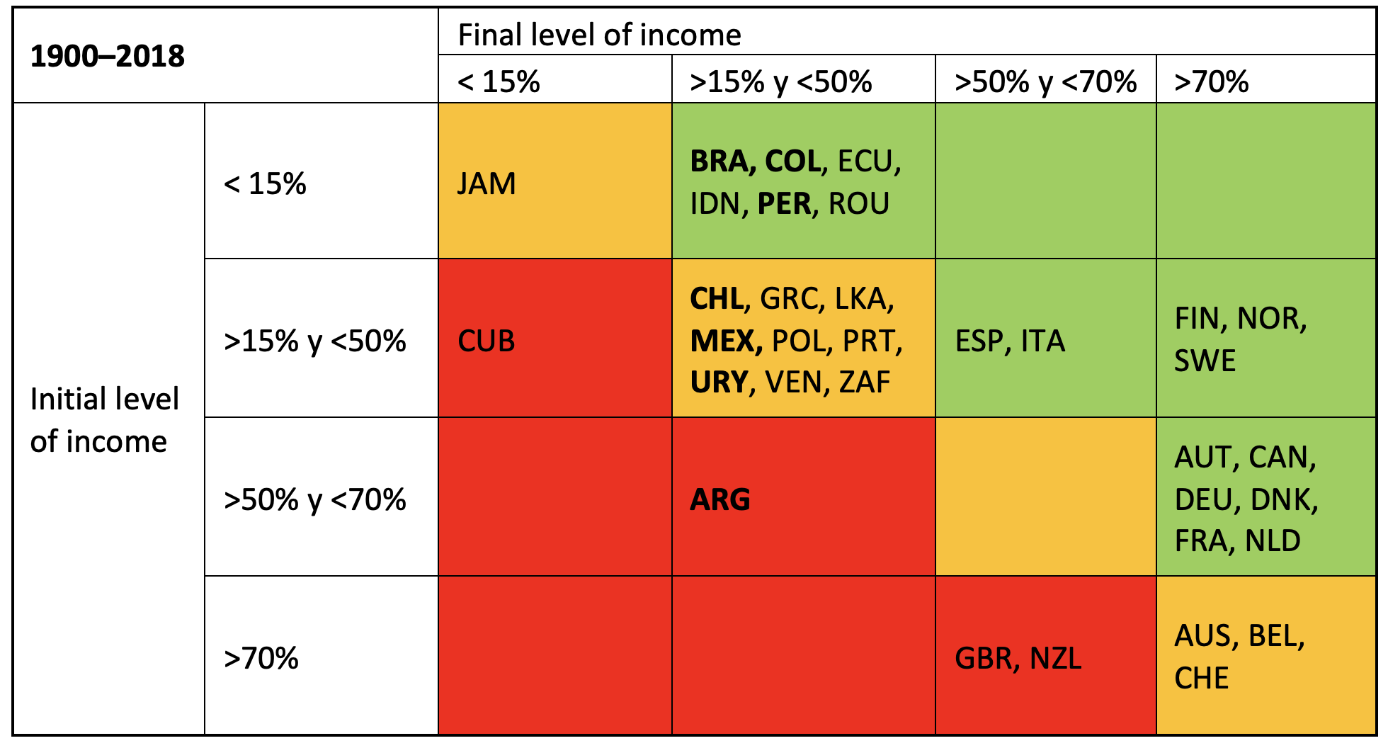
Another way to illustrate Argentina’s exceptionality is to look at the per capita income transition matrix, namely, the probability of moving between different stages of per capital income within a given time span. Following Arias and Wen (2015), we estimate the transition matrix between per capita income levels relative to the US, which we take as a reference of the income frontier. Unlike these authors, who focus on transitions over short (and moving) time windows (which implies that they have several observations for any given country), we compare the beginning-to-end transition within the entire period under study (1900 to 2018), giving us one observation per country.
We define four relative income brackets: low (less than 15% of the US per capita income), lower middle (15% to 50%), upper middle (50% to 70%), and high (more than 70%). We assign countries to the transition matrix according to their ‘departure’ and ‘arrival’ positions.
In Table 1, the diagonal (in yellow) represents countries that remained in the same group. Green boxes represent ‘successful’ transitions: convergence to a higher bracket in the income scale. Red boxes (below the diagonal) illustrate ‘unsuccessful’ transitions: long-term divergence. As can be seen, there are only a handful of countries in the initial sample that fall in the red areas: Cuba, which moved from lower-middle-income to low-income; the UK and New Zealand, which both moved from high-income to upper-middle-income; and Argentina, which moved from upper-middle-income to middle-income.
Table 1 Transition matrix of income levels 1900–2018
Source: Own elaboration based on Maddison Project Database (2020).
An unstable plateau
Argentina’s peculiar divergence story includes a final chapter characterised by a slower relative decline, albeit with a marked increase in both real and nominal volatility.
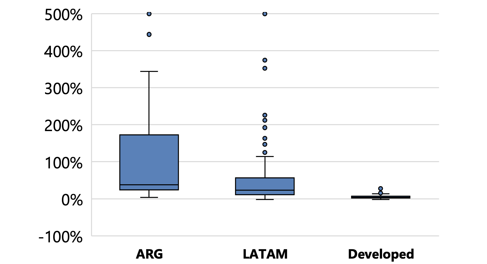
Figure 5 shows that the relative volatility of the real growth rate of Argentina compared with the reference countries almost doubled after 1990, when the divergence began to plateau.
Interestingly, the same pattern is also apparent with respect to neighbouring countries.
Figure 5 Volatility of the real growth rate of Argentina
a) Relative to benchmark countries
b) Relative to Latin American countries
Source: Own elaboration based on Maddison Project Database (2020).
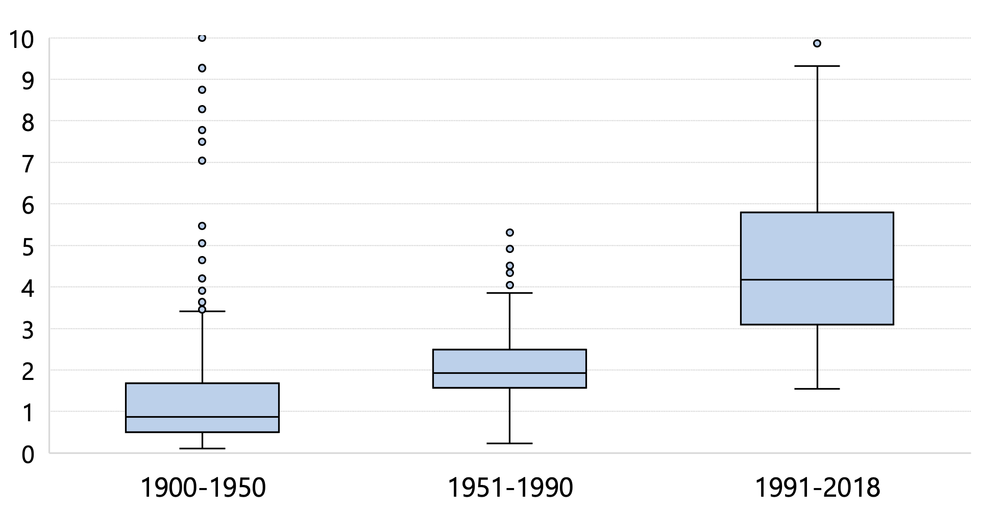
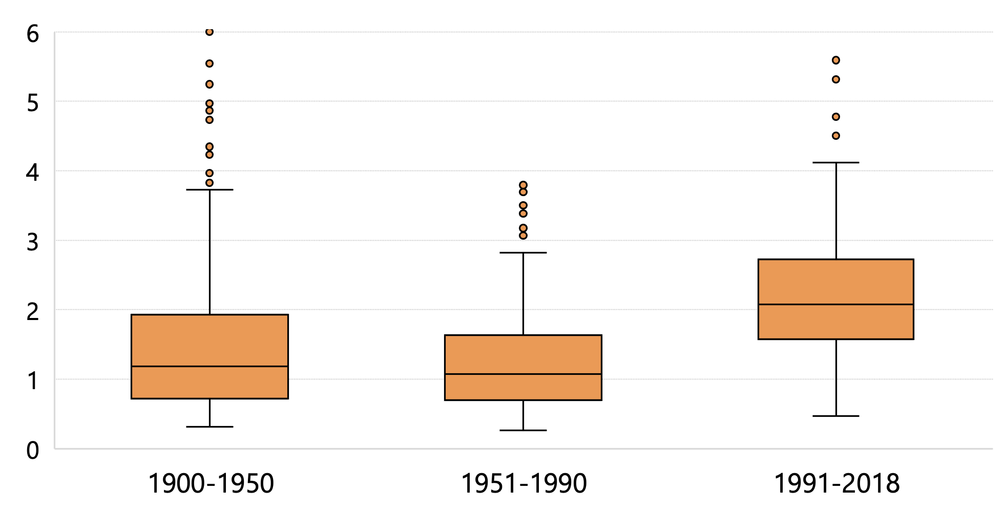
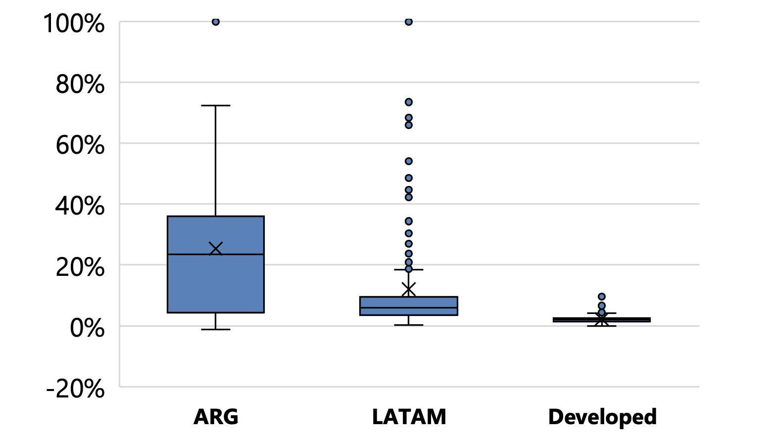
This higher real volatility coincided with a visible increase in relative inflation levels: while Argentina had exhibited high inflation (and bouts of hyperinflation) historically, particularly in the post-Bretton Woods period, this has also been the case for other Latin American economies, as indicated by the comparable median inflation rates. However, since the 1990s, even in the absence of hyperinflation episodes, the median inflation rate was 20% higher than its neighbours’, making the contrast more visible: at a time when Latin American economies embraced nominal stability, Argentina was still swamped by chronic and volatile inflation (Figure 6).
Figure 6 Distribution of annual inflation rates
a) 1950-1990
b) 1991-2023
Source: Own elaboration based on Gerchunoff and Llach (1998), INDEC, Statistics Bureau of Buenos Aires City, Statistics Bureau of San Luis, IMF, Central Bank of Brazil, and Central Bank of Chile.
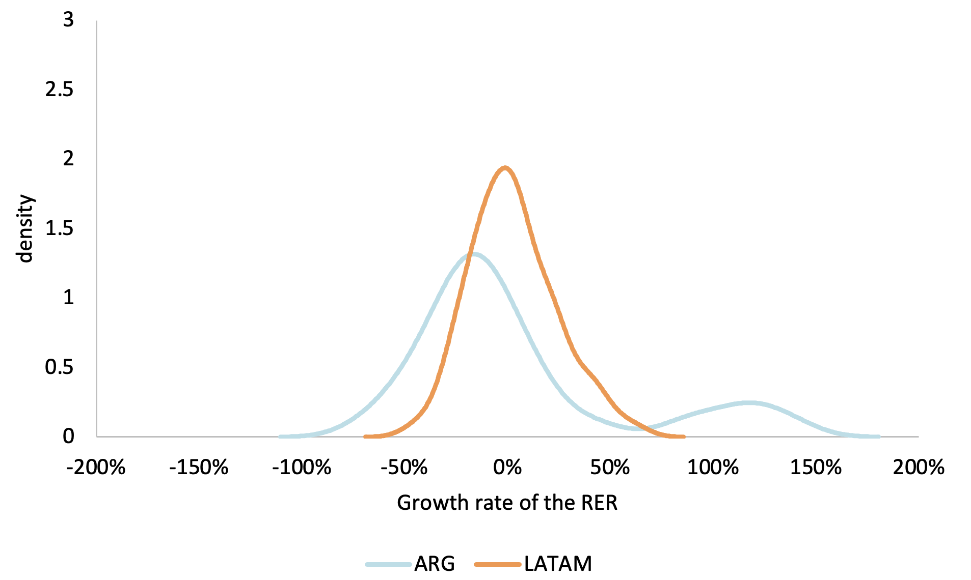
This tension between slow growth and chronic inflation has led the country to resort to the exchange rate anchor as a substitute for more conventional monetary and fiscal policies, with the predictably short-lived dividends ending in discrete exchange rate realignments. As a result, the real exchange rate has exhibited an unusual pattern, with long periods of (gradual and ultimately unsustainable) overvaluation followed by sharp corrections, often to the point of overshooting – presumably, a good starting point for the next exchange rate anchor experiment. Thus, an asymmetric, bi-modal distribution arises, whereby the real exchange rate is (usually) overvalued or (occasionally) sharply undervalued, but seldom stays close to the mean, as opposed to neighbouring countries, where the distribution is closer to normal with virtually no fat tails (Figure 9).
Figure 7 Five-year variation of the official USD multilateral real exchange rate, kernel density plot (1991–2023 period)
Source: Own elaboration based on IMF, BCRA, and Central Bank Reserve of Peru.
Note: Kernel density with gaussian smoothing; bandwidths selected through Silverman’s (1986) rule of thumb.
Final remarks
Our findings are consistent with a narrative that emphasises a secular divergence (with some circumstantial incidents, such as WWII and a brief pause in the 1960s) converging ‘from above’ to a middle-income trap (Foxley 2012). Alternatively, one could argue in favour of a post-war decoupling story, particularly if we dismiss the initial peak as an epiphenomenon resulting from a spasmodic development process that anticipated the immigration waves. In both cases, the evidence questions the popular idea that the decline began in the 1970s, when the country’s domestic market-driven productive pattern became unsustainable, both fiscally and externally, deepening a chronic foreign exchange shortage (Gerchunoff 2022). While this decline is visible in the data, it is hard to argue that the divergence started at such a late date.
In turn, the secular divergence narrative sheds new light on the political consequences of divergence. Do the social demands behind the chronic fiscal imbalance reflect the memory of a rich (at the beginning of the century) and egalitarian (post-war) society? How does a protracted economic deterioration feed into governments’ spending anxiety? To what extent does a society that reaches middle income levels from above differ from Latin American societies that did the same from below? These are all important questions for future research.
References
Arias, M A and Y Wen (2015), “Trapped: Few Developing Countries Can Climb the Economic Ladder or Stay There”, The Regional Economist 23(4), October.
Bai, J and P Perron (1998), “Estimating and Testing Linear Models with Multiple Structural Changes”, Econometrica 66: 47–78.
Bolt, J and J Luiten van Zanden (2020), “Maddison style estimates of the evolution of the world economy: A new 2020 update”, Maddison-Project Working Paper WP-15.
De Long, J B (1988), “Productivity Growth, Convergence, and Welfare: Comment”, American Economic Review 78(5): 1138–54.
Foxley, A (2012), La Trampa del Ingreso Medio. El desafío de esta década para América Latina, Santiago de Chile: CIEPLAN.
Gerchunoff, P (2022), “El nudo argentino: Una nueva justicia social para un nuevo patrón de crecimiento”, Le Monde Diplomatique, May.
Katz, S and E Levy Yeyati (2024), “When did Argentina lose its mojo? A short note on economic divergence”, Working paper 1/2024.
Llach, L (2020), “Rica, pero no tan moderna: Argentina antes de la Depresión”, Desarrollo Económico 60(231): 153–79.
Pritchett, L (1997), “Divergence, Big Time”, Journal of Economic Perspectives 11(3): 3–17.

