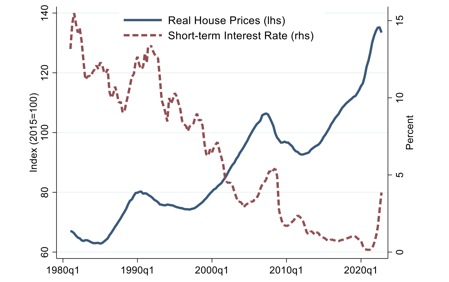
Real house price growth in OECD countries further accelerated after the onset of the Covid-19 pandemic, from an already steep upward trend that began in the early 2010s (Figure 1). Yet, soon after, housing markets were confronted with the fastest monetary tightening in decades. A casual glance at the data, as well as an abundant theoretical literature, would suggest that a cooling – or even a substantial contraction – is on the cards. The conceptual argument often involves non-arbitrage conditions: first, between renting and owning (Poterba 1984, Henderson and Ioannides 1983); and second, between investing in housing rather than in other assets (Case and Shiller 1989, 1990). Yet, these non-arbitrage conditions have been shown to be substantially weaker in reality than in theory (Glaeser and Gyourko 2009, Duca et al. 2021), leaving the link between interest rates and house prices a predominantly empirical question.
Figure 1 House prices and short-term interest rates (lhs: 2015=100, rhs: in %)
Note: Unweighted averages of real house price indices and the money market or treasury bill rates, respectively, over 29 OECD countries. 1980Q1 – 2022Q4. Sources: OECD.
In a recent paper (Burgert et al. 2024), we provide new evidence on how house prices react to monetary policy rates and how this reaction depends on the underlying cyclical conditions in the housing market and the broader economy. For this, we rely on the experience of 29 OECD countries over four decades. Relative to focusing on the experience of an individual country, this allows us to exploit a far larger number of monetary and housing cycles as well as a more diverse set of initial conditions.
We identify exogenous variations in domestic policy rates based on monetary policy spillovers from the US, in the spirit of Jordà et al. (2015).
The instrumentation strategy relies on the idea that – conditional on an accurate description of domestic conditions – a tightening of monetary conditions in the financial centre increases the likelihood of a domestic policy hike, in line with the international ‘policy dilemma’ proposed by Rey (2015). We further allow the effect of interest rates to differ across a range of economic indicators, relying on the smooth transition functions (STFs) popularised by Auerbach and Gorodnichenko (2012).
Key results
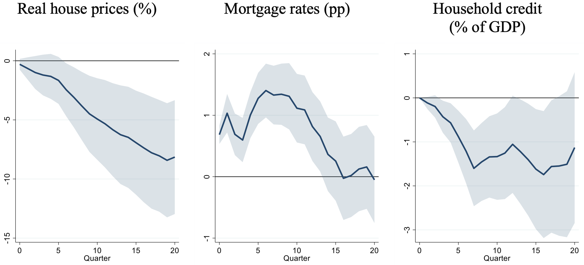
Our key findings are the following. First, we find that following an exogenous one percentage point increase in short-term interest rates, house prices typically fall by up to 8% over a five-year period (Figure 2, left). This effect materialises through a substantial transmission to typical mortgage rates (Figure 2, centre) and a persistent decline in private credit (Figure 2, right). Compared to the existing literature, which – according to a meta-study by Ehrenbergerova et al. (2023) – suggests an average peak house-price reaction of 1.2% after just two years, our response is substantially larger and more protracted. In the paper, we show that this difference is predominantly due to our identification of monetary policy shocks, and the fact that the endogenous component of an interest rate hike, such as an overheating economy, risks attenuating the identified effect.
Figure 2 Monetary policy’s effect on house prices and its transmission
Note: The figure shows the IRFs of real house prices (in %), typical mortgage rates (in pp), and household credit (in % of GDP) to a one percentage point increase in short-term interest rates. The shaded area corresponds to the 90% confidence interval. Robust standard errors clustered at the country level.
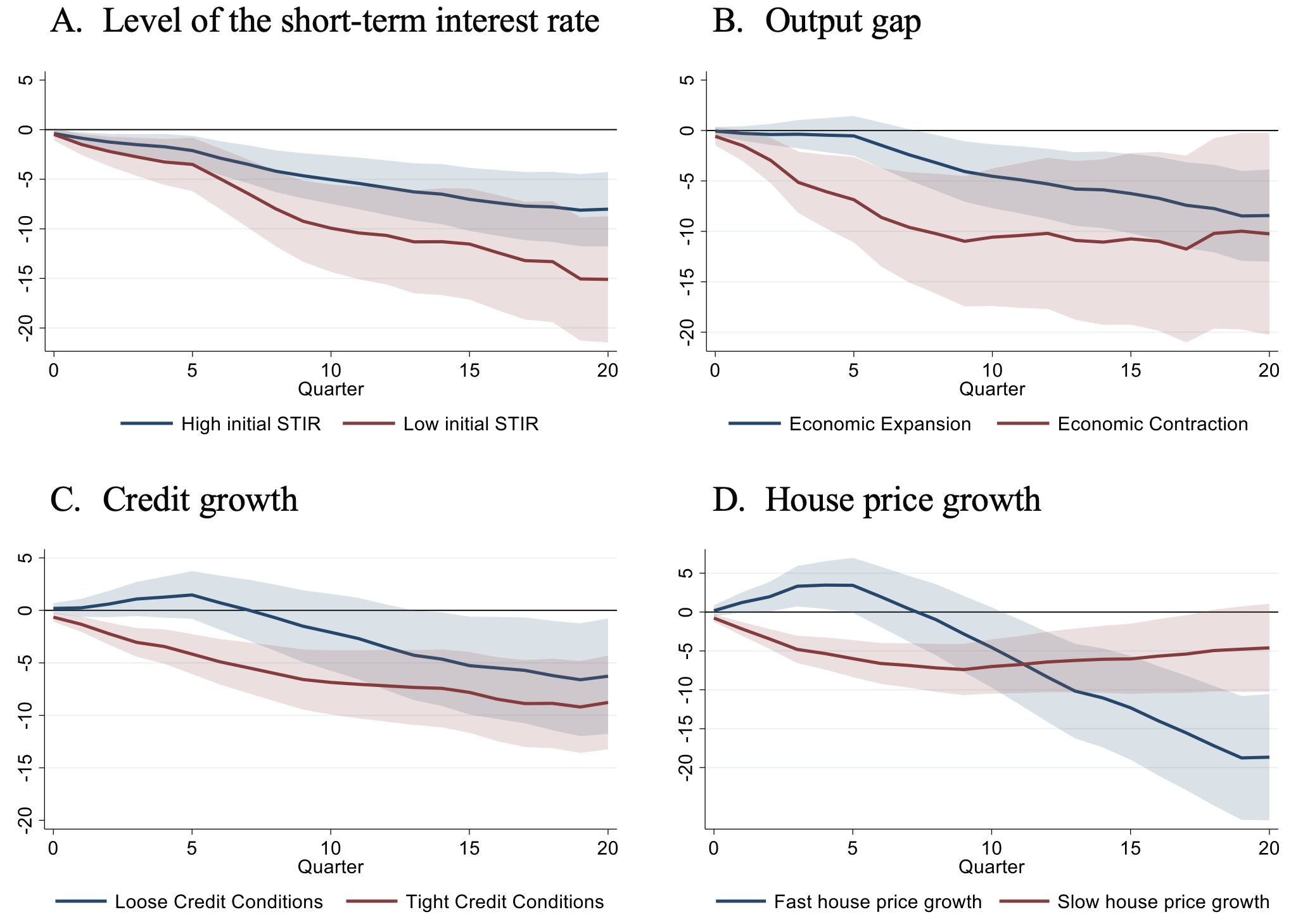
Second, we find that the effect on house prices varies substantially with initial conditions. For example, the response of house prices is substantially larger when interest rates are initially low (Figure 3A), and they materialise faster when their rise occurs in a recession (Figure 3B) or when credit conditions are already tight (Figure 3C). A preceding house price boom slows price reactions at the outset but amplifies them in the medium-term (Figure 3D).
Figure 3 House price reaction depending on cyclical conditions
Note: The figure shows the IRFs of house prices to a one percentage point increase in short-term interest rates depending on the underlying conditions, captured by the level of the smooth transition function, constructed with a trailing seven-quarter moving average of globally standardised variables. The red curve (low state) corresponds to the STF taking a value of 0.8. The blue curve (high state) corresponds to STF=0.2. The shaded area corresponds to the 90% confidence interval.
Implications for the ongoing tightening cycle
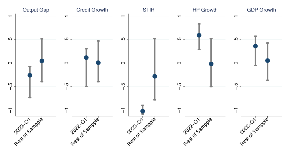
Finally, we illustrate the possible implications of our results by conditioning the house price reaction on the economic context at the onset of the latest monetary tightening cycle (i.e. in 2022Q1). For the average economy, these were characterised by extraordinarily low short-term interest rates, a broadly neutral credit cycle, a slightly positive real cyclical position (in terms of GDP growth),
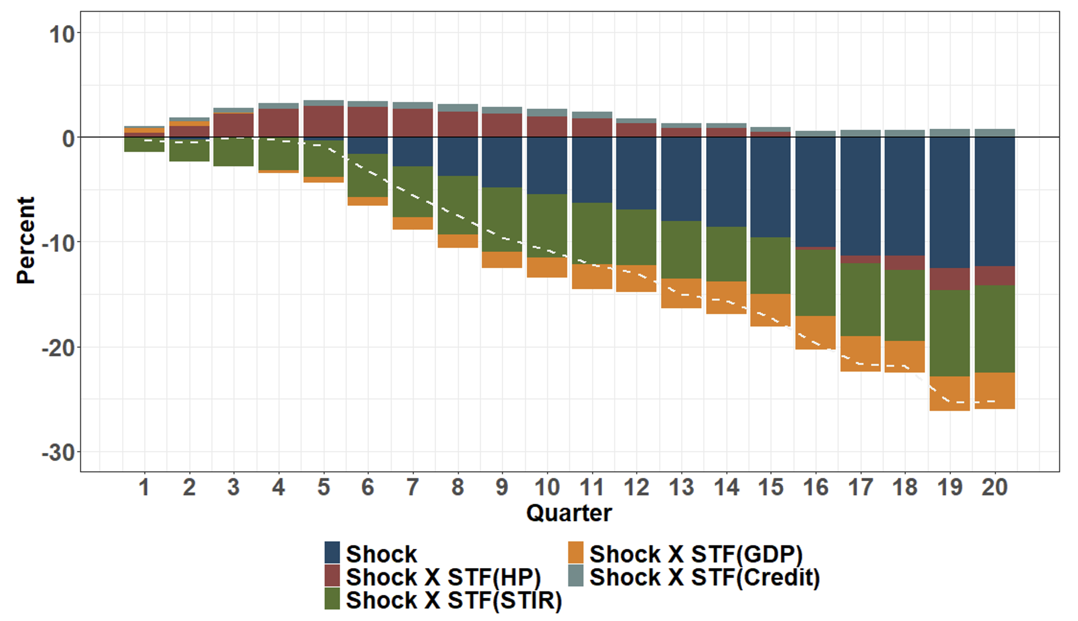
and unusually dynamic house price growth (Figure 4). Estimating jointly the influence of these factors, we find that historically they contributed to attenuating the house price reaction in the short-term but amplified its impact in the medium-term (Figure 5).
Figure 4 The cyclical conditions in 2022-Q1
Note: The figure shows the median and the interquartile range of the 2022-Q1 and the average values of the standardised seven-quarter MA of the output gap, the growth of household credit (in % of GDP), the level of the short-term interest rate and the growth in real house prices.
Figure 5 The semi-elasticities of house prices in 2022-Q1
Note: The figure shows the average model-implied semi-elasticity of house prices to a one percentage point increase in short-term interest rates given the cyclical conditions of 2022-Q1, captured by the level of the smooth transition function of GDP growth (GDP), credit growth (Credit), the level of the short-term interest rate (STIR), and the past house price growth (HP). The shaded area corresponds to the 90% confidence interval.
The estimated house price semi-elasticity, given the conditions in 2022-Q1, is above 25. This is an order of magnitude bigger than the average effect from the existing literature. Yet, two comments are in order. First, our coefficients show the effect of an exogenous one percentage point shock to the policy rate. Clearly, much of the observed change does not satisfy such a criterion and was considered endogenous, both by market participants and by our model. Second, the estimation coefficient shows the effect, conditional on the rich dynamics in our model. The identified effect should thus be interpreted as a deviation from the counterfactual path of house prices and not as a deviation from the level of house prices at time t.
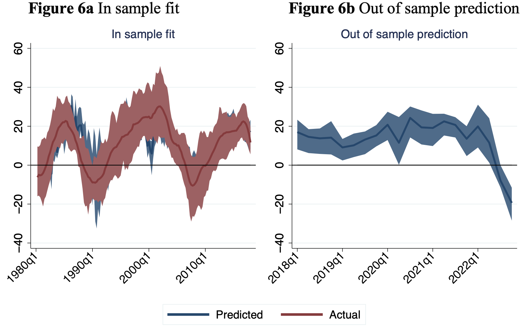
These caveats notwithstanding, historical patterns still suggest that the medium-term outlook deteriorated substantially with the most recent tightening. We illustrate this with the predicted 20-quarter forward growth rate. Over the in-sample period, the predicted and actual growth rates follow each other very closely (Figure 6a). The out-of-sample prediction, which is shown in Figure 6b (and starts in 2018 due to the forward-looking horizon), is first broadly stable but deteriorates significantly during the course of 2022. Under the strong assumption that no further interest rate innovations will take place going forward – implying a very sluggish normalisation of monetary policy – our model would predict a real house price contraction between 12% and 28% (i.e. the interquartile range) over the period ending in 2027.
Note: The figures compare the actual 20-quarter forward growth rate (change in the log) of real house prices (in blue) with the predicted change based on our model over the same horizon. The shaded area corresponds to the interquartile range.
The objective of this column is not to make predictions about where house prices are heading. After all, the pandemic-related shifts in housing-related preferences, strong household balance sheets, and more pronounced supply constraints may provide more persistent upward pressure on house prices than our model can capture. However, the analysis does emphasise that house price reactions to monetary tightening in the past have often been sluggish but large, particularly when initial cyclical conditions resembled those of 2022. In addition, our paper echoes the conclusion from a growing literature emphasising the state contingency of monetary policy transmission (e.g. Tenreyro and Thwaites 2016, Barnichon and Matthes 2018, Debortoli et al. 2020).
References
Auerbach, A J and Y Gorodnichenko (2012), “Measuring the Output Responses to Fiscal Policy”, American Economic Journal: Economic Policy 4(2): 1–27.
Barnichon, R and C Matthes (2018), “Functional Approximation of Impulse Responses”, Journal of Monetary Economics 99(C): 41–55.
Burgert, M, J Eugster and V Otten (2023), “Interest rate sensitivity of house prices: International evidence on its state dependence”, Working Paper, Swiss National Bank, forthcoming.
Case, K and R Shiller (1989), “The Efficiency of the Market for Single-Family Homes”, American Economic Review 79(1): 125–37.
Case, K and R Shiller (1990), “Forecasting Prices and Excess Returns in the Housing Market”, Journal of Real Estate Finance and Economics 18(4).
Debortoli, D, M Forni, L Gambetti and L Sala (2020), “Asymmetric Effects of Monetary Policy Easing and Tightening”, CEPR Discussion Paper 15005.
Duca, J V, J Muellbauer and A Murphy (2021), “What Drives House Price Cycles? International Experience and Policy Issues”, Journal of Economic Literature 59(3): 773–864.
Ehrenbergerova, D, J Bajzik and T Havranek (2023), “When Does Monetary Policy Sway House Prices? A Meta-Analysis”, IMF Economic Review 71(2): 538–73.
Glaeser, E L and J Gyourko (2009), “Arbitrage in Housing Markets”, Housing Markets and the Economy: Risk, Regulation, and Policy, 113–46.
Henderson, J V and Y M Ioannides (1983), “A Model of Housing Tenure Choice”, American Economic Review 73(1): 98–113.
Jordà, Ò, M Schularick and A M Taylor (2015), “Betting the house”, Journal of International Economics 96(S1): 2–18.
Poterba, J M (1984), “Tax Subsidies to Owner-Occupied Housing: An Asset Market Approach”, Quarterly Journal of Economics 99(4): 729–52.
Rey, H (2015), “Dilemma not Trilemma: The Global Financial Cycle and Monetary Policy Independence”, NBER Working Paper 21162.
Tenreyro, S and G Thwaites (2016), “Pushing on a String: US Monetary Policy Is Less Powerful in Recessions”, American Economic Journal: Macroeconomics 8(4): 43–74.
