The neutral rate of interest – or r-star – is one of the most important concepts for monetary policy, as it provides a navigation star for central bankers’ interest rate policies (Powell 2018). The concept was first introduced by Wicksell (1898) and describes the hypothetical level of the real rate of interest that sets the economy’s growth rate at its potential and inflation at its target value. As the neutral rate of interest cannot be observed, it has to be estimated.
One of the most widely used estimates for r-star is by Laubach and Williams (2003), whose recent re-publication of estimates after a two-year hiatus due to the Covid-19 shock (Holston et al. 2023) sparked a vivid debate about the usefulness of the estimate on social media. Apart from the fact that one of the most important reference variables for monetary policy was not available precisely at a time when uncertainties were greatly increased by a major shock, the changes in the estimation procedure altered the entire time series up to the 1960s, in some cases considerably.
This latest criticism joins an existing literature that has produced various criticisms of the neutral interest rate estimation method. This includes for example the strong and persistent downward trend since the 1960s. Buncic (2021) shows that this downward trend is mainly driven by an autoregressive random walk term whose implementation suffers from serious econometric weaknesses. The persistent downward trend is also influenced by the high values of r-star in the 1960s, that are only present in the estimations by Laubach and Williams (2003) and Holston et al. (2017) but not in most other estimates.
Another criticism concerns the output gaps estimated by Laubach and Williams. Before the financial crises there was a clear overlap between these estimates and official estimates from the Congressional Budget Office. However, since the financial crises a large and persistent gap has emerged between the two series of up to seven percentage points.
While Laubach and Williams describe the theoretical determination of the neutral rate of interest with a simple Keynesian model, they estimate it based on a golden rule state in a standard neoclassical growth model, i.e. with a fundamentally different theoretical framework. In a recent paper (Bofinger and Haas 2023), we provide an approach to estimate the neutral rate of interest based on a Keynesian model as described by Laubach and Williams. We utilise a simple New Keynesian macro model where the central bank sets its interest rate in a way that minimises the output gap y and the deviation of the inflation rate π from its target value. The central bank thus follows a loss function that includes the inflation gap and the output gap. Both terms are squared, since the objectives are symmetric, and a preference parameter weights the relative importance of the two terms.
Using this loss function, we can observe neutral periods, i.e. periods where the overall loss is close to zero. Under the assumption that this is an indication of an absence of exogenous shocks, it is possible to derive a proxy for the neutral rate during these periods. We assume that in such neutral periods, the actual real policy rate is close to the neutral rate. From these observed manifestations of the neutral rate, we compute a moving average to smooth the adjustments between different manifestations. In non-neutral periods, we cannot observe new manifestations of the neutral rate and therefore insert the latest value of our averaged time series.
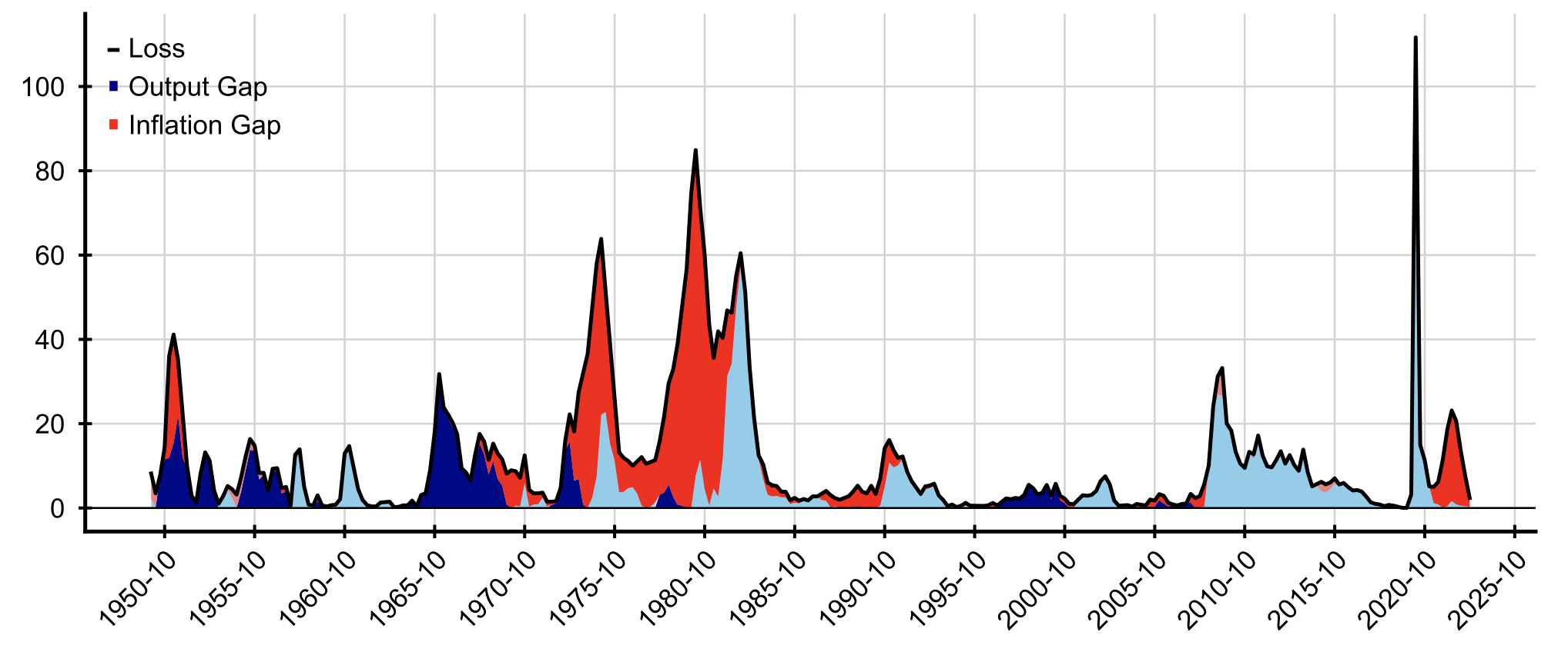
Figure 1 shows a loss function for the US economy. The loss function does a good job of capturing the evolution of the US economy over the past 70 years. The 1960s were a fairly stable period with low inflation. This is followed by a period of high inflation in the 1970s and early 1980s, the reaction of the Volcker Fed which brought inflation down but also a recession, the period of great moderation with low losses, the financial crises with rather persistent losses, and the Covid recession followed by high inflation rates.
Figure 1 Loss function for the US
Notes: This figure shows a loss function for the US. Lighter colouring indicates negative gaps, darker colouring indicates positive gaps (Source: FRED).
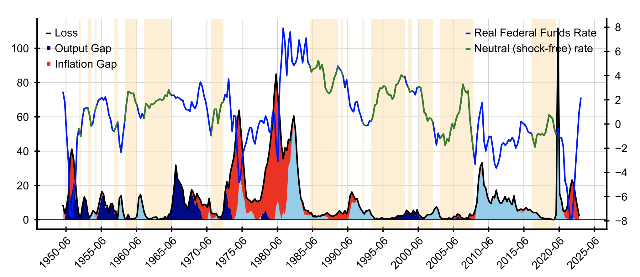
If we add the real federal funds rate to that figure and set the threshold for neutral periods equal to five, we can directly derive values for our measure for the neutral rate of interest (Figure 2).
Figure 2 Real policy rate and neutral rate for the US
Notes: This figure presents the loss function for the US and the real Federal Funds rate. Shaded areas are neutral phases with a loss less than or equal to five.
Source: FRED.
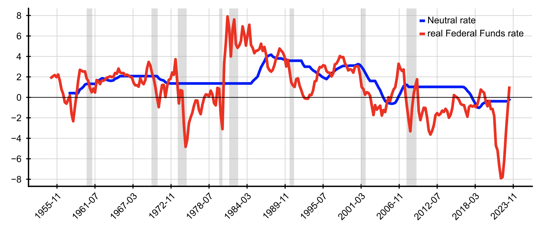
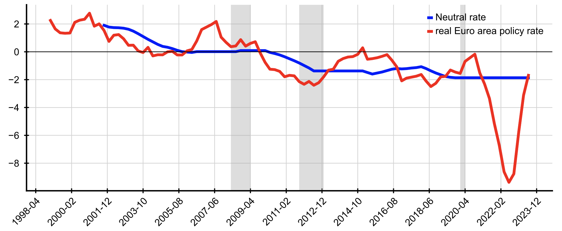
As described above, we compute a moving average of the observed values of the neutral rate of interest to account for its character as a medium- to long-term concept. The neutral rate can be used to assess the monetary policy stance. Figure 3 shows the neutral rate for the US (upper panel) and the euro area (lower panel) and the corresponding real policy rates. In both cases, we find a prolonged period of loose monetary policy in the years leading up to the financial crisis, followed by an abrupt tightening just before the onset of the crisis. Our measure of the neutral rate is also insensitive to the extreme but brief Covid-19 recession, suggesting that it is mainly a temporary shock for the time being.
Figure 3 The neutral rate and the real policy rate
A) United States
B) Euro area
Notes: This figure shows the neutral rate and real policy rates for the US (Panel A) and the euro area (Panel B). Shaded areas indicate recession phases.
Source: FRED, ECB, OECD.
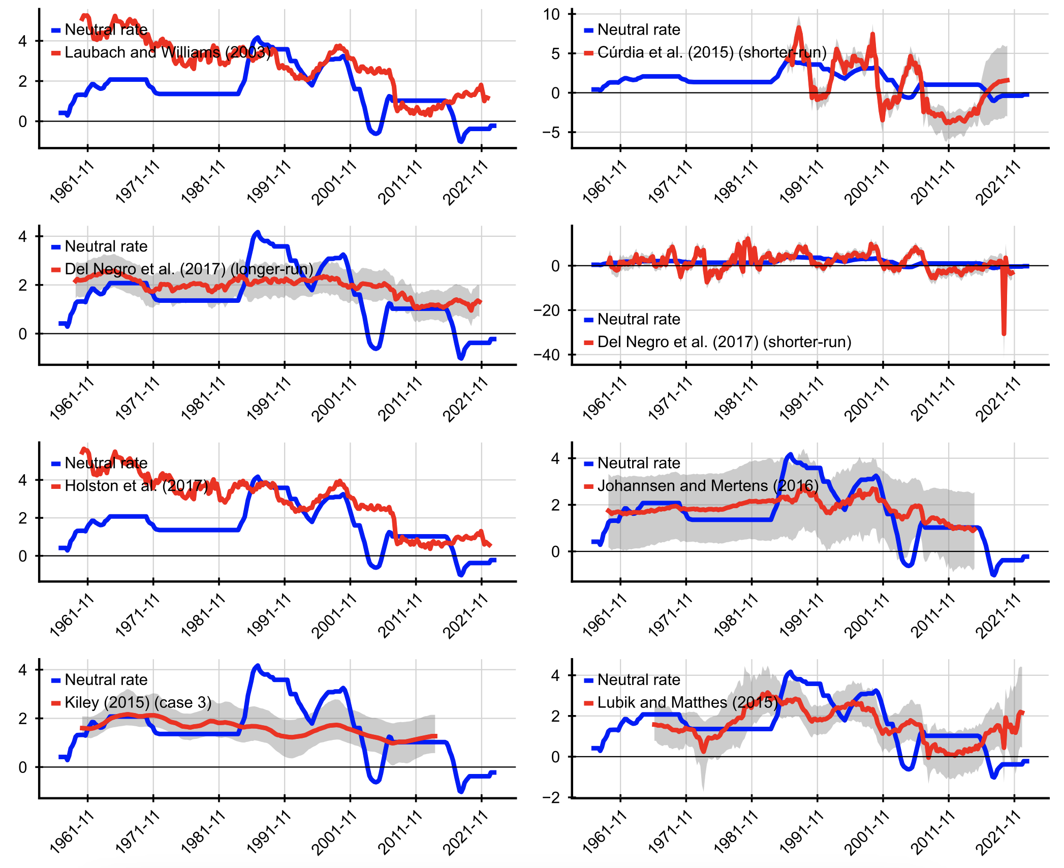
Our measure of the neutral rate of interest shows a remarkable overlapping with many other estimations of a neutral rate of interest, as Figure 4 shows. Figure 4 also highlights the high uncertainty of the r-star estimates, with confidence bands of up to two percentage points around the mean or median estimate. Our neutral rate measure often lies within the confidence bands of other measures, implying that the estimates are statistically indistinguishable. In line with all other measures except for Laubach and Wlliams (2003) and Holston et al. (2023), we do not find evidence for a secular decline in the neutral rate of interest. This is also in line with empirical data for net returns on the net capital stock for most advanced economies.
Figure 4 Comparison between the neutral rate and alternative measures for r-star
Notes: This figure shows the neutral rate and different measures for r-star. Confidence bands are added when available
Source: Laubach and Williams (2003), Holston et al. (2017), Johannsen and Mertens (2016), Del Negro et al. (2017), Lubik and Matthes (2015), Kiley (2015, case 3 scenario), Cúrdia et al. (2015).
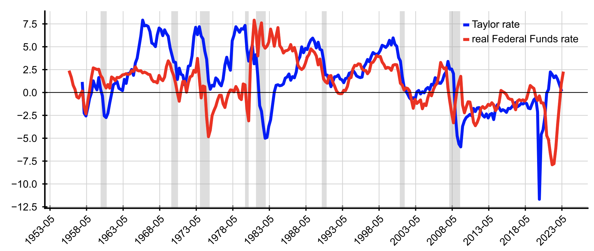
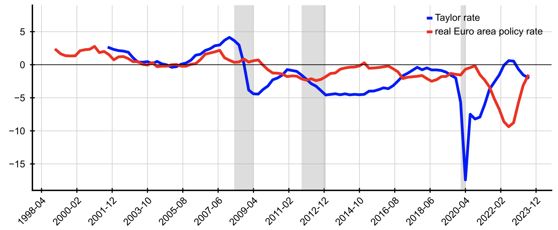
Finally, to test the performance of our neutral rate measure for a monetary policy heuristic, we estimate a Taylor rule using our neutral rate. Figure 5 shows the Taylor rates for the US and the euro area together with the real policy rates.
Figure 5 Taylor rates based on the neutral rate and real policy rates
A) United States
B) Euro area
Notes: This figure shows the Taylor rate for the US (upper panel) and the euro area (lower panel) based on neutral rate. Shaded areas indicate recession phases.
Source: Fred, ECB, OECD.
The upper panel in Figure 5 shows that our Taylor rate is in fact very close to the actual real federal funds rate since 1987. In fact, for the period 1987 to 1992 Taylor (1993) discovered his famous rule. Deviations in the late 1960s and 70s, when the actual real federal funds rate was well below the Taylor rate, were followed by high rates of inflation. Similarly, in the early 1980s, the Taylor rate was well below the real federal funds rate, suggesting that monetary policy was too restrictive at the time. The period preceding the housing crisis also shows a deviation from the Taylor rule signalling a too expansionary monetary policy. For the euro area we find similar deviations for the period preceding the financial crisis. For the period of the euro crisis and the following years we find a too restrictive monetary policy, which may have contributed to the rather slow recovery.
Despite its simplicity, our methodology is based on a consistent theoretical derivation from a simple New Keynesian model and largely corresponds to existing approaches to determine r-star. Considering that r-star is a purely theoretical concept and that all approaches to its measurement suffer from very high uncertainty with confidence bands up to six percentage points, a simple calculation has its advantages.
References
Bofinger, P and T Haas (2023), “R-Star: A new approach to estimate the polar star of monetary policy”, CEPR Discussion Paper No. 18420.
Buncic, D (2021), “Econometric issues with laubach and williams’ estimates of the natural rate of interest”, Sveriges Riksbank Working Paper Series, No. 397.
Cúrdia, V, A Ferrero, G C Ng and A Tambalotti (2015), “Has us monetary policy tracked the efficient interest rate?”, Journal of Monetary Economics 70: 72–83.
Del Negro, M, D Giannone, M P Giannoni and A Tambalotti (2017), “Safety, liquidity, and the natural rate of interest”, Brookings Papers on Economic Activity 2017(1): 235–316.
Holston, K, T Laubach and J C Williams (2017), “Measuring the natural rate of interest: International trends and determinants”, Journal of International Economics 108: S59–S75.
Holston, K, T Laubach and J C Williams (2023), “Measuring the natural rate of interest after covid-19”, Federal Reserve Bank of New York Staff Reports, No. 1063.
Johannsen, B K and E Mertens (2016), “The expected real interest rate in the long run: Time series evidence with the effective lower bound”, FEDS Notes, Washington: Board of Governors of the Federal Reserve System, 9 February.
Kiley, M T (2015), “What can the data tell us about the equilibrium real interest rate?”, Finance and Economics Discussion Series 2015-077, Washington: Board of Governors of the Federal Reserve System.
Laubach, T and J C Williams (2003), “Measuring the natural rate of interest”, Review of Economics and Statistics 85(4): 1063–1070.
Lubik, T A and C Matthes (2015), “Calculating the natural rate of interest: A comparison of two alternative approaches”, Richmond Fed Economic Brief.
Powell, J H (2018), “Monetary policy in a changing economy”, At "Changing Market Structure and Implications for Monetary Policy", a symposium sponsored by the Federal Reserve Bank of Kansas City, Jackson Hole, Wyoming, August.
Taylor, J B (1993), “Discretion versus policy rules in practice”, Carnegie-Rochester conference series on public policy 39:195–214.
Wicksell, K (1898), Interest and prices, Mises Institute.
