In the wake of the financial crisis of 2008 and 2009, central banks have cut policy rates to near zero in order to contain the decline in economic activity and prevent deflation. Eight years on, nominal interest rates are still at low levels, inflation is well below central banks’ targets, and output growth is muted. The narrative of policymakers justifying such policies also remains broadly unchanged.
According to the existing paradigm, central banks have leverage over the real economy because firms find it costly to adjust prices in response to temporary changes in monetary policy. But is this channel still effective when monetary policy is persistent? Or should we be looking at other channels? We argue that the sticky price channel loses its potency when interest rates are kept at the same level for a long time. Instead, monetary policy starts to transmit through long-term nominal debt contracts such as mortgages or instalment loans. However, the real effects working through this channel in a traditional macro model are mainly redistributive.
The sticky price channel
The sticky price channel is the central mechanism of monetary policy transmission in the modern macro literature. A number of texts (e.g. Woodford 2003, Galí 2015) describe this channel in detail.1 The key element of this channel is the so-called ‘New-Keynesian Phillips curve’. According to this relationship, aggregate output depends negatively on the expected change in the inflation rate. If today’s inflation is high relative to tomorrow’s expected inflation – that is, the expected change in inflation is negative – aggregate output is relatively high today. The microeconomic foundations for this relationship are driven by the costly adjustment of prices at the firm level. Consider a firm that faces a cost of adjusting its price. When the aggregate price level increases, and thus inflation increases, the firm finds itself with a higher demand, as its products look relatively cheap. If the increase in the aggregate price level is expected to only be temporary, the firm does not find it profitable to incur the adjustment cost of changing its price. Instead, it increases output to satisfy the higher demand. In equilibrium, all firms facing price adjustment costs behave this way and, as a result, aggregate output increases. However, when the increase in inflation is expected to be highly persistent, the cost of changing the price is worth paying and the firm adjusts its price, rather than output. In equilibrium, all firms behave this way and, as a result, aggregate output does not change. The sticky price channel is thus most potent when changes in policy rates, and thus inflation, are only temporary.
The mortgage channel
The mortgage channel works through changes in the real value of the regular mortgage payments homeowners have to make over the life of a loan. Contractually, mortgage payments are set in nominal terms and their exact form depends on the type of the loan. Most mortgage loans are derived from two basic contracts:
- Fixed-rate mortgages (FRMs); and
- Adjustable-rate mortgages (ARMs).
An FRM is defined as a mortgage with the nominal interest rate fixed for at least ten years, and often for the entire term of the loan (15-30 years). An ARM is defined as a mortgage whose nominal interest rate can change from one period to another, usually in line with some short-term nominal interest rate, such as the policy rate set by the central bank.
Since mortgages are long-term loans, changes in the policy rate and inflation affect the real cost, to homeowners, of new loans (the so-called ‘price effect’), as well as the real value of payments on the outstanding debt (the so-called ‘income effect’).2 In an earlier paper (Garriga et al. 2013), we make this distinction explicit. Here, we focus only on the income effect, which is the more relevant effect for consumption, a variable we want to focus on in this column.
The direction of monetary policy effects working through the mortgage channel depends on the nature of mortgage contracts in each country. With ARMs, the real value of the payments on outstanding mortgage debt is affected, first and foremost, by the short-term nominal interest rate. The short-term nominal interest rate determines the nominal payments while inflation translates the nominal payments into real payments. However, because mortgage loans amortise very slowly (over 15-30 years) the effect of the change in the nominal interest rate charged on the outstanding debt dominates any effect of inflation on the real value of the payments. A decline in the short-term nominal interest rate, even when accompanied by a one-for-one decline in the inflation rate, reduces real mortgage payments. This way, low nominal interest rates redistribute income from savers/mortgage investors to mortgage borrowers.
In contrast, with FRMs, nominal payments are fixed. Real payments on outstanding mortgage debt can thus only be affected by inflation. A decline in inflation increases the real value of the mortgage payments, with the quantitative effect depending on how persistent the decline in inflation is. A more persistent decline in inflation has a larger effect than a temporary decline because over time the effect of accumulated low inflation increases the real value of the payments more and more. As a result, persistently low inflation redistributes income from mortgage borrowers to savers/investors and the size of the redistribution increases over time. In some countries (such as the US), refinancing of FRMs is possible. As a result, the response to an interest rate decline falls somewhere in between the ARM and FRM cases.
Quantitative comparison of the two channels
In recent research, we quantitatively compare the two channels of monetary policy transmission in a calibrated dynamic general equilibrium model, assuming alternative degrees of persistence of the short-term nominal interest rate controlled by monetary policy (Garriga et al. 2016). The baseline experiment explores the responses of the model economy to a one-percentage point (annualised) decline in the short-term nominal interest rate. Here we reproduce only a few of the results, focusing on consumption (in the paper, we also investigate the effects on housing and non-housing investment and output).
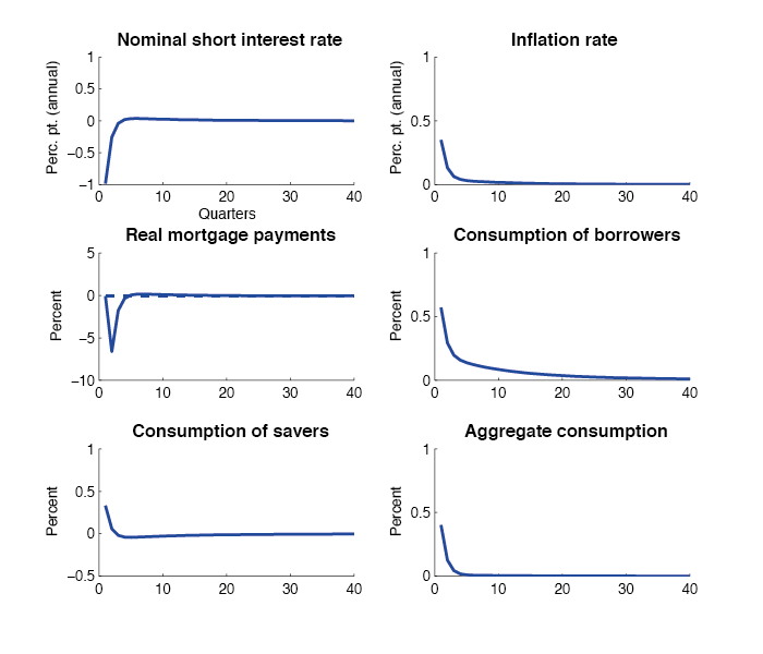
In the experiment summarised in Figure 1, the persistence of the decline, an autocorrelation of 0.3, is calibrated so as to be consistent with the responses of the short rate to standard monetary policy shocks identified by the VAR literature. In line with the VARs, and New-Keynesian models, inflation increases (the real rate thus declines). As the increase in inflation is expected to be temporary, output – and thus consumption – increase in response to the shock, for the reasons discussed above. The increase in consumption is experienced by both borrowers and savers. The borrowers’ consumption, however, increases by more (as a percentage from steady state) than that of savers, as borrowers are assumed to be less able to smooth out changes in income than savers.3 The responses are almost identical for FRMs and ARMs. The reason for this is that, as shown in the figure, with ARMs changes in mortgage payments are only temporary (due to the decline in the short rate), while with FRMs the short-lived increase in inflation has only a negligible effect on real mortgage payments (dashed line), leaving them essentially unchanged. The responses shown in the figure are therefore almost entirely attributed to sticky prices; mortgages are nearly irrelevant when changes in the policy rate are as temporary as in this example.
Figure 1. Effects of temporary changes in the policy rate on ARMs and FRMs
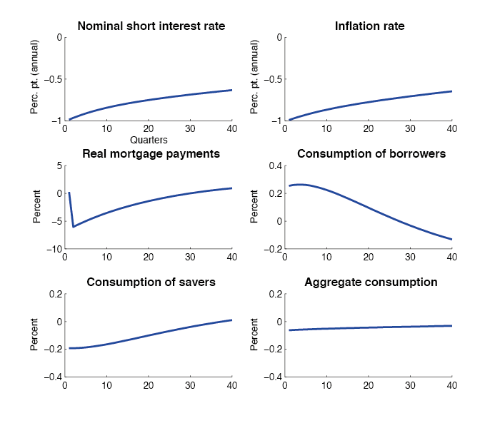
Figure 2, in contrast, shows the responses to a highly persistent decline in the short rate, an autocorrelation of 0.99. In this case, due to the Fisher effect, inflation declines almost as much as the short rate, leaving the real rate essentially intact. Yet, with ARMs, real mortgage payments decline on impact about as much as in the case of the temporary shock. In the present case, however, the decline is much more persistent. In response to this boost in disposable income, borrowers’ consumption persistently increases, though, on impact, quantitatively less than in the case of the temporary shock. The gain for borrowers is a loss for savers, whose consumption declines, but less than that of borrowers. In the paper we show that the responses are almost entirely due to the mortgage channel. As the decline in inflation is very persistent, the sticky price channel plays only a small role for the reasons discussed above. In the context of a standard macroeconomic model, aggregate consumption thus changes only little and the effect of the shock is mainly re-distributive.
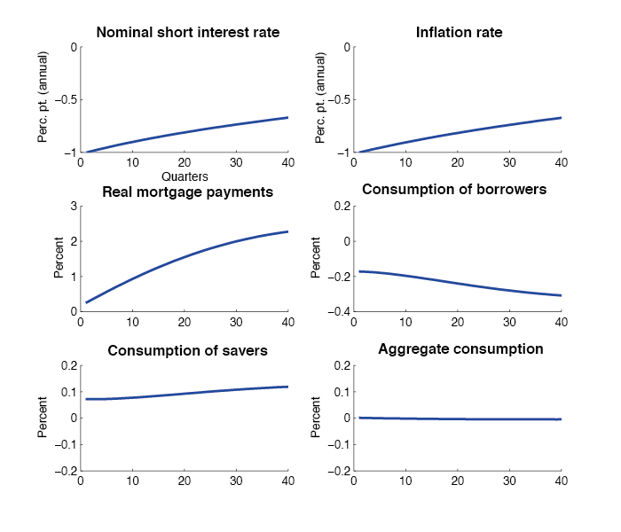
With FRMs, as Figure 3 shows, the persistently low inflation increases the real value of mortgage payments, but – as discussed above – this effect takes time. In this case, borrowers lose while savers gain, leaving aggregate consumption again almost intact.4
Figure 2. Effects of highly persistent changes in the policy rate on ARMs
Figure 3. Effects of highly persistent changes in the policy rate on FRMs
Empirical relevance of temporary versus persistent policy rate changes
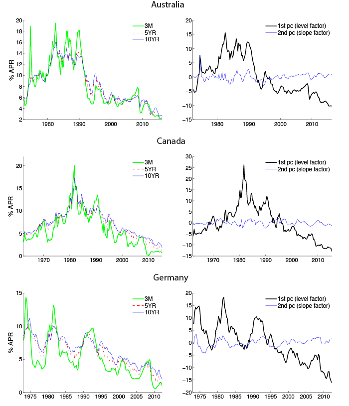
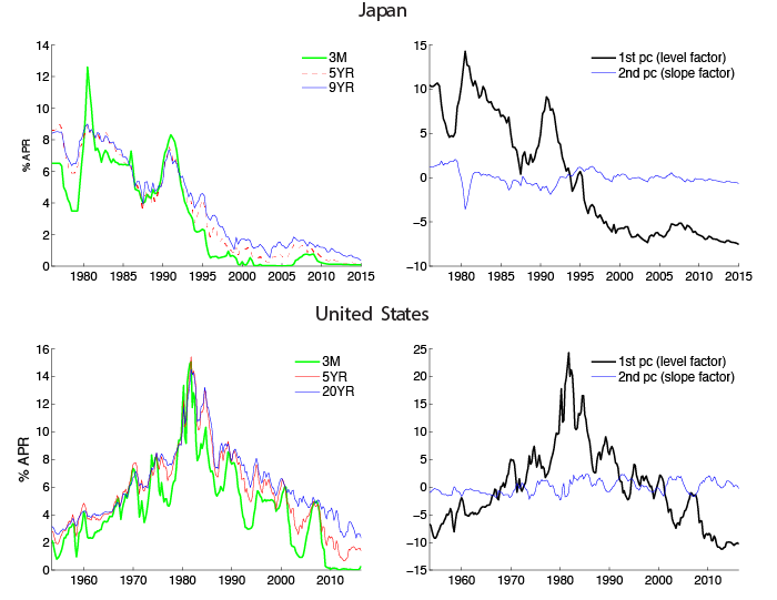
Which one of these two channels is empirically more relevant, given the observed movements of interest rates? For the ease of comparison, in the above computational experiments the decline in the short rate has been normalised to be one percentage point (annualised) for both temporary and persistent changes. To gauge the typical sizes of temporary and persistent movements in the observed short rate, we employ the principal component analysis of the nominal yield curve (see Piazzesi 2006). Figures 4 and 5 show selected yields on government bonds of different maturities for a number of countries and their first two principal components. Together, the two principal components account for essentially all of the fluctuations in the yields, regardless of the maturity.5 It is apparent from the figures that the first principal component dominates the movements in interest rates, statistically accounting for about 95% of the movements in the short rate. The first principal component is also highly persistent, with an autocorrelation of about 0.98, close to the autocorrelation of the persistent changes in the short rate in our computational experiments.
When we calibrate the size of the temporary and persistent changes in the short rate in the model to match the volatility of the two principal components, the redistributive effects on consumption demonstrated above turn out to be somewhat larger than the aggregate effects, when measured by the unconditional volatility of percentage deviations of aggregate and individual consumption from steady state. The size of redistribution is similar for FRMs and ARMs, although the timing and direction are different (in line with our discussion above).
Figure 4. Nominal interest rates and principal components
Figure 5. Nominal interest rates and principal components (cont.)
Policy implications
Our findings have clear implications for the current policy environment, in which nominal interest rates have been kept at low levels for almost a decade. The purpose of such policies was to stimulate aggregate economic activity. According to our model, the initial cut in policy rates may have fulfilled this objective, to the extent it was expected to be temporary, but the subsequent policy of keeping rates low for a substantial period of time more likely led to income and consumption redistribution than to the desired aggregate effects. As inflation followed nominal interest rates to similarly low levels, based on our model, we can infer that lenders in predominantly FRM countries (the US, Germany, France, Belgium) gained at the expense of borrowers due to persistently low inflation rates, while in predominantly ARM countries (most other countries) borrowers gained at the expense of lenders due to persistently low nominal interest rates.
References
Bernanke, B S and M Gertler (1995) “Inside the black box: The credit channel of monetary transmission”, Journal of Economic Perspectives, 9: 27–48.
Galí, J (2015) Monetary policy, inflation, and the business cycle: An introduction to the New Keynesian framework and its applications, third edition, Princeton University Press.
Garriga, C, F E Kydland and R Šustek (2013) “Mortgages and monetary policy”, NBER, Working Paper 19744.
Garriga, C, F E Kydland and R Šustek (2016) “Nominal rigidities in debt and product markets”, NBER, Working Paper 22613.
Mishkin, F (2007) “Housing and the monetary transmission mechanism”, Finance and Economics Discussion Series 2007-40, Federal Reserve Board.
Piazzesi, M (2006) “Affine term structure models”, in Y Ait-Sahalia and L P Hansen, (eds), Handbook of Financial Econometrics, Elsevier, Amsterdam.
Rupert, P and R Šustek (2016) “On the mechanics of New-Keynesian models”, Centre for Macroeconomics, Discussion Paper 1608.
Woodford, M (2003) Interest and prices: Foundations of a theory of monetary policy, Princeton University Press.
Endnotes
[1] These texts focus on models without capital accumulation and thus without aggregate saving. Rupert and Šustek (2016) put the sticky price channel under scrutiny in the context of a model with capital accumulation. Our description of the sticky price transmission mechanism applies to both environments.
[2] The income effect is sometimes referred to in the literature as the cash flow or household balance sheet effect (Bernanke and Gertler 1995, Mishkin 2007).
[3] In the model, mortgage borrowers represent the typical middle-class homeowner, while savers represent the top quintile of the wealth distribution; both supply labour but only savers invest in non-housing capital, more or less in line with the data (the model is calibrated to be consistent with the basic cross-sectional properties of the data).
[4] In some countries, such as the US, FRM borrows can refinance relatively easily, taking advantage of declines in interest rates. In Garriga et al (2013) we take such refinancing explicitly into account. But when calibrated to the data, refinancing activity turns out not to be large enough to change the basic arguments made here.
[5] The figure shows only a few selected yields as examples; the principal component analysis is carried out for a broad spectrum of maturities.


